Руководство пользователя — FieldView (FieldView.exe)
Программа: Tamic Rt Output Field Viewer (внутреннее имя проекта — FldView, исполняемый файл
FieldView.exe, версия 4.1). Интерфейс программы англоязычный — в руководстве приводятся английские названия пунктов как в программе, а рядом — русское пояснение. Подписи на скриншотах русские.
1. Назначение программы
FieldView — это вьювер (программа просмотра) распределения поля пакета TMC Suite. Счётные ядра PlanarRT_H и PlanarRT_X во время электродинамического расчёта сохраняют «карты» поля в расчётной области, а FieldView рисует эти карты в виде двумерных цветных картин или трёхмерных поверхностей (с помощью OpenGL).
Простыми словами: ядро посчитало, как поле распределено по плоскости модели, и записало это в файл; FieldView открывает такой файл и показывает его как картинку — где поле сильнее, где слабее, как оно устроено внутри рупора, линзы, резонатора и т. п.
Программа умеет показывать три независимых «слоя» (layer) одной и той же области, каждый со своими настройками цвета и отрисовки:
| Слой | Что показывает |
|---|---|
| Field (Поле) | основное распределение поля из открытого файла; |
| Eps (ε) | распределение диэлектрической проницаемости среды; |
| Topology (Топология) | геометрия модели и её границы (металл, поглотитель, диэлектрик, вход, магнитная стенка). |
Это MDI-программа: в одном окне можно открыть сразу несколько файлов поля и сравнивать их (меню Window).
2. Запуск программы и открытие данных
- Запустите файл
FieldView.exe(папкаdist/win32/bin/илиdist/win64/bin/). Откроется главное окно. - Откройте файл поля: меню File → Open… (или кнопка
 на панели инструментов, или
 Ctrl+O). - В диалоге выбора файла укажите файл одного из поддерживаемых типов —
.tf,.AMPили.FAZ(например,samples/SAMPLE_R/1/quasi0.AMP). Подробно о форматах — раздел 8. - После открытия имя файла появится в заголовке окна:
Tamic Rt Output Field Viewer - [quasi0.AMP]. - Поле отрисуется в рабочей области. Если изображения не видно — проверьте включён ли слой Field
(кнопки 22–23 на панели или меню View → Field) и нажмите View → Default (
Ctrl+D), чтобы вернуть стандартный масштаб и положение.
Можно запустить программу сразу с файлом: перетащите
.AMP/.FAZ/.tfна значок программы или передайте путь аргументом командной строки:FieldView.exe "путь\к\файлу.AMP".
3. Главное окно
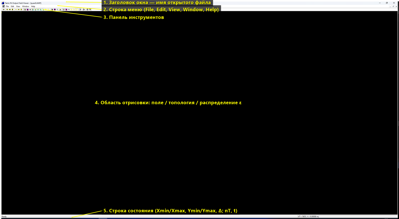
Главное окно состоит из пяти зон (показаны цифрами на рисунке в разделе 1):
| № | Зона | Назначение |
|---|---|---|
| 1 | Заголовок окна | Название программы и имя открытого файла. |
| 2 | Строка меню | Все команды: File, Edit, View, Window, Help. |
| 3 | Панель инструментов | Кнопки быстрого доступа к самым частым командам (35 кнопок). |
| 4 | Область отрисовки | Здесь OpenGL рисует поле / топологию / распределение ε. Управляется мышью и клавишами (масштаб, поворот, сдвиг). |
| 5 | Строка состояния | Слева — служебные сообщения и текущие границы вида (Xmin/Xmax, Ymin/Ymax, Delta); справа — параметры открытого файла (nT — номер шага, t — время). |
О скриншотах области отрисовки. Часть обзорных картинок этого руководства сделана в среде, где содержимое окна OpenGL не попадает в снимок экрана, поэтому область отрисовки (зона 4) на них выглядит чёрной. На реальном компьютере здесь отображается цветная картина поля (примеры «живого» результата —
main-window-field.png,field-3d.png,eps-layer.png).
4. Панель инструментов
Панель инструментов дублирует самые нужные команды. Кнопки слева направо пронумерованы 1–35 и сгруппированы (группы разделены вертикальными промежутками):

| № | Кнопка | Команда | Клавиша | Что делает |
|---|---|---|---|---|
| 1 | |
File → Open | Ctrl+O |
Открыть файл поля (.tf/.AMP/.FAZ/.ex). |
| 2 |  |
Zoom + | + |
Увеличить масштаб (по обеим осям). |
| 3 |  |
Zoom +X | X |
Увеличить масштаб только по оси X. |
| 4 |  |
Zoom +Y | Y |
Увеличить масштаб только по оси Y. |
| 5 |  |
Zoom − | − |
Уменьшить масштаб (по обеим осям). |
| 6 |  |
Zoom −X | Shift+X |
Уменьшить масштаб по оси X. |
| 7 |  |
Zoom −Y | Shift+Y |
Уменьшить масштаб по оси Y. |
| 8 |  |
Topology → Line | Shift+L |
Слой топологии: рисовать линиями (каркас). |
| 9 |  |
Topology → Surface | Shift+S |
Слой топологии: рисовать заливкой (поверхностью). |
| 10 |  |
Topology → Dimension 2/3 | Shift+D |
Переключить топологию между 2D и 3D. |
| 11 |  |
Boundary → Eps | E |
Подсветить границы диэлектрика (ε). |
| 12 |  |
Boundary → Metal | M |
Подсветить границы металла. |
| 13 |  |
Boundary → Magnetic | N |
Подсветить границы магнитной стенки. |
| 14 |  |
Boundary → Absorber | A |
Подсветить границы поглотителя. |
| 15 |  |
Boundary → Input | I |
Подсветить границы входа (порта). |
| 16 |  |
Topology → Dimensions → Block | K |
Показать размеры/нумерацию блоков. |
| 17 |  |
Topology → Dimensions → Link_List | Alt+K |
Показать размеры по списку связей (Link List). |
| 18 |  |
Eps → Line | Alt+L |
Слой ε: рисовать линиями. |
| 19 |  |
Eps → Surface | Alt+S |
Слой ε: рисовать заливкой. |
| 20 |  |
Eps → Dimension 2/3 | Alt+D |
Переключить ε между 2D и 3D. |
| 21 |  |
Eps → Size | Alt+J |
Авторазмер слоя ε по оси Z (высота). |
| 22 |  |
View → Eps → Type → Eps+ | — | Режим величины: показывать проницаемость ε (обычный режим, доступен всегда). |
| 23 |  |
View → Eps → Type → N | — | Плазма (X‑мода): показывать концентрацию электронов N. Доступна, только если в данных есть плазма (блоки RECT_STAT_N). |
| 24 |  |
View → Eps → Type → B | — | Плазма (X‑мода): показывать внешнее магнитное поле B (подмагничивание). Доступна при наличии блоков RECT_STAT_B. |
| 25 |  |
View → Eps → Type → Y | — | Плазма (X‑мода): показывать потери Y. Доступна при наличии блоков RECT_STAT_Y. |
| 26 |  |
Field → Line | L |
Слой поля: рисовать линиями. |
| 27 |  |
Field → Surface | S |
Слой поля: рисовать заливкой. |
| 28 |  |
Field → Dimension 2/3 | D |
Переключить поле между 2D и 3D. |
| 29 |  |
Size → along an X axies | Ctrl+J |
Показать размерную сетку вдоль оси X. |
| 30 |  |
Size → along an Y axies | Shift+J |
Показать размерную сетку вдоль оси Y. |
| 31 |  |
Field → Size | J |
Авторазмер слоя поля по оси Z (высота рельефа). |
| 32 |  |
View → Proportionally | P |
Включить/выключить пропорциональный масштаб осей X и Y. |
| 33 |  |
View → Default | Ctrl+D |
Сбросить вид к стандартным параметрам. |
| 34 |  |
File → Print | Ctrl+P |
Печать текущего изображения. |
| 35 |  |
Help → About | — | О программе (версия). |
Кнопки 22–25 (EPS · N · B · Y) — новые. Это переключатель отображаемой величины для расчётов плазмы (X‑мода,
tmc_rtx): E (жёлтая) — проницаемость ε; N (красная) — концентрация электронов; B (синяя) — магнитное поле подмагничивания; Y (зелёная) — потери. Кнопки N, B, Y активны (цветные), только когда в открытом поле присутствует соответствующая плазма; иначе они серые (неактивные). Подробнее — раздел 5.3.2.1.Подсказка: при наведении курсора на кнопку в программе всплывает её английское название, а в строке состояния показывается короткое описание.
Чистый вид панели без нумерации:

5. Меню
5.1. File (Файл)
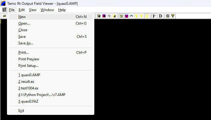
| Пункт | Перевод | Клавиша | Действие |
|---|---|---|---|
| New | Создать | Ctrl+N |
Новый пустой документ. |
| Open… | Открыть | Ctrl+O |
Открыть файл поля (.tf/.AMP/.FAZ). |
| Close | Закрыть | — | Закрыть текущий документ. |
| Save | Сохранить | Ctrl+S |
Сохранить документ. |
| Save As… | Сохранить как | — | Сохранить под другим именем. |
| Print… | Печать | Ctrl+P |
Печать изображения. |
| Print Preview | Предпросмотр печати | — | Предварительный просмотр перед печатью. |
| Print Setup… | Параметры печати | — | Выбор принтера и параметров страницы. |
| (список 1, 2, 3…) | Недавние файлы | — | Быстрое открытие недавно использованных файлов. |
| Exit | Выход | — | Закрыть программу. |
5.2. Edit (Правка)
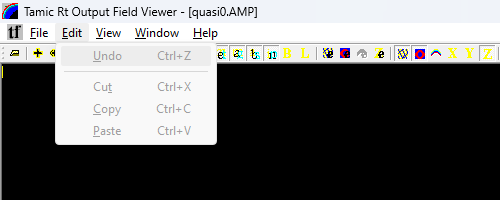
| Пункт | Перевод | Клавиша | Действие |
|---|---|---|---|
| Undo | Отменить | Ctrl+Z |
Стандартная команда (в текущем режиме недоступна — серая). |
| Cut / Copy / Paste | Вырезать / Копировать / Вставить | Ctrl+X / Ctrl+C / Ctrl+V |
Команды буфера обмена (недоступны — серые). |
В этой версии меню Edit не задействовано: программа только просматривает данные, не редактирует их.
5.3. View (Вид)
Главное меню управления отображением. Содержит вызов окна параметров, три подменю слоёв (Topology / Eps / Field), подменю управления видом (Zoom / Rotate / Translate) и переключатели.
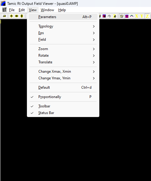
| Пункт | Перевод | Клавиша | Действие |
|---|---|---|---|
| Parameters | Параметры | Alt+P |
Открыть окно настроек вида (раздел 6.1). |
| Topology ► | Топология | — | Подменю слоя топологии (5.3.1). |
| Eps ► | Диэлектрик ε | — | Подменю слоя ε (5.3.2). |
| Field ► | Поле | — | Подменю слоя поля (5.3.3). |
| Zoom ► | Масштаб | — | Подменю масштабирования (5.3.4). |
| Rotate ► | Поворот | — | Подменю поворота (3D) (5.3.5). |
| Translate ► | Сдвиг | — | Подменю сдвига сцены (5.3.6). |
| Change Xmax, Xmin ► | Сдвиг окна по X | — | Сдвиг видимого диапазона по X (5.3.7). |
| Change Ymax, Ymin ► | Сдвиг окна по Y | — | Сдвиг видимого диапазона по Y (5.3.7). |
| Default | По умолчанию | Ctrl+d |
Сбросить вид к стандартным параметрам. |
| Proportionally | Пропорционально | P |
Сохранять одинаковый масштаб осей X и Y (галочка = включено). |
| Toolbar | Панель инструментов | — | Показать/скрыть панель инструментов. |
| Status Bar | Строка состояния | — | Показать/скрыть строку состояния. |
5.3.1. View → Topology (слой топологии)
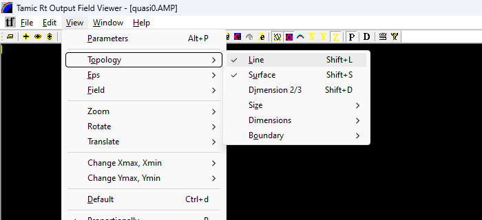
| Пункт | Клавиша | Действие |
|---|---|---|
| Line | Shift+L |
Рисовать топологию линиями (каркас). |
| Surface | Shift+S |
Рисовать топологию заливкой. |
| Dimension 2/3 | Shift+D |
Переключить 2D 3D. |
| Size ► | — | Размерная сетка вдоль осей (5.3.1.1). |
| Dimensions ► | — | Показ размеров блоков / списка связей (5.3.1.2). |
| Boundary ► | — | Подсветка границ материалов (5.3.1.3). |
5.3.1.1. Topology → Size — размерная сетка:
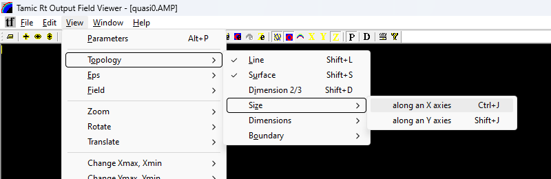
- along an X axies (
Ctrl+J) — нанести размеры вдоль оси X; - along an Y axies (
Shift+J) — нанести размеры вдоль оси Y.
5.3.1.2. Topology → Dimensions — показ размеров элементов:
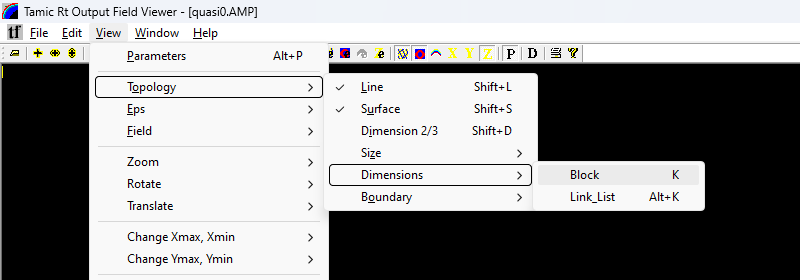
- Block (
K) — размеры/нумерация блоков; - Link_List (
Alt+K) — размеры по списку связей (Link List).
5.3.1.3. Topology → Boundary — подсветка границ материалов (галочка = слой включён):
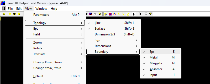
- Eps (
E) — границы диэлектрика; - Metal (
M) — границы металла; - Magnetic (
N) — границы магнитной стенки; - Absorber (
A) — границы поглотителя; - Input (
I) — границы входа (порта возбуждения).
5.3.2. View → Eps (слой диэлектрика)
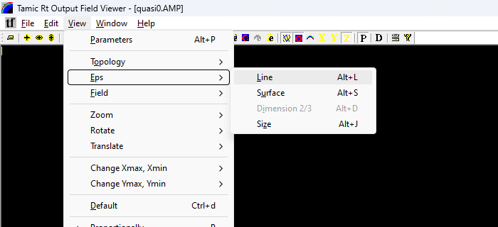
| Пункт | Клавиша | Действие |
|---|---|---|
| Line | Alt+L |
Рисовать ε линиями. |
| Surface | Alt+S |
Рисовать ε заливкой. |
| Dimension 2/3 | Alt+D |
Переключить 2D 3D (в текущей версии может быть серым). |
| Size | Alt+J |
Авторазмер слоя ε по оси Z. |
| Type ► | — | Выбор отображаемой величины: ε / N / B / Y (плазма). См. 5.3.2.1. |
5.3.2.1. View → Eps → Type — отображаемая величина (плазма X‑моды)
Подменю Type (и новые кнопки панели инструментов 22–25) выбирают, какую физическую
величину рисовать в слое «Eps» для расчётов плазмы в X‑моде (ядро tmc_rtx):
| Пункт меню | Кнопка | Величина | Когда доступно |
|---|---|---|---|
| Eps+ | — E, жёлтая |
Диэлектрическая проницаемость ε (обычный режим) | Всегда |
| N | — N, красная |
Концентрация электронов плазмы N, м⁻³ | Только если в поле есть блоки RECT_STAT_N |
| B | — B, синяя |
Внешнее магнитное поле подмагничивания B, Тл | Только если есть блоки RECT_STAT_B |
| Y | — Y, зелёная |
Потери плазмы Y | Только если есть блоки RECT_STAT_Y |
Как пользоваться. Откройте поле, посчитанное X‑ядром с плазмой (файл .ex/.tf рядом с
топологией .tt, где заданы блоки RECT_STAT_N/_B/_Y), затем нажмите нужную кнопку (или пункт
меню). Слой «Eps» переключится с обычной ε на выбранную величину. Если в данных плазмы нет,
кнопки N/B/Y серые (неактивные) — доступен только Eps+. Выбранный режим запоминается
между запусками.
Величины N, B, Y соответствуют блокам
RECT_STAT_N(концентрация электронов, м⁻³),RECT_STAT_B(магнитное поле подмагничивания, Тл) иRECT_STAT_Y(потери) в шаблоне задачи.tpl— см. руководство по ядру PlanarRT_X.
5.3.3. View → Field (слой поля)
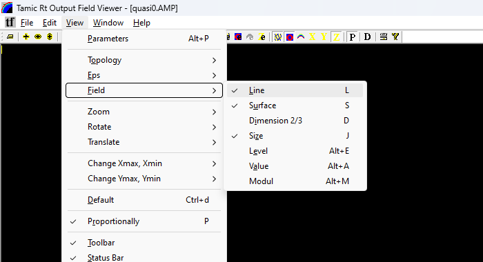
| Пункт | Клавиша | Действие |
|---|---|---|
| Line | L |
Рисовать поле линиями. |
| Surface | S |
Рисовать поле заливкой. |
| Dimension 2/3 | D |
Переключить 2D 3D. |
| Size | J |
Авторазмер слоя поля по оси Z (высота рельефа). |
| Level | Alt+E |
Открыть окно выбора уровней цвета (раздел 6.3). |
| Value | Alt+A |
Режим показа числового значения поля под курсором. |
| Modul | Alt+M |
Показывать модуль поля. |
5.3.4. View → Zoom (масштаб)
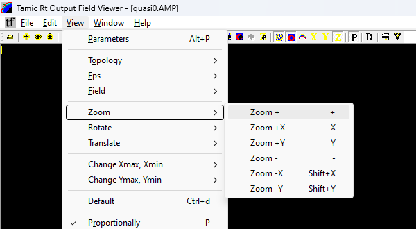
| Пункт | Клавиша | Действие |
|---|---|---|
| Zoom + | + |
Увеличить (обе оси). |
| Zoom +X | X |
Увеличить по X. |
| Zoom +Y | Y |
Увеличить по Y. |
| Zoom − | − |
Уменьшить (обе оси). |
| Zoom −X | Shift+X |
Уменьшить по X. |
| Zoom −Y | Shift+Y |
Уменьшить по Y. |
5.3.5. View → Rotate (поворот, для 3D)
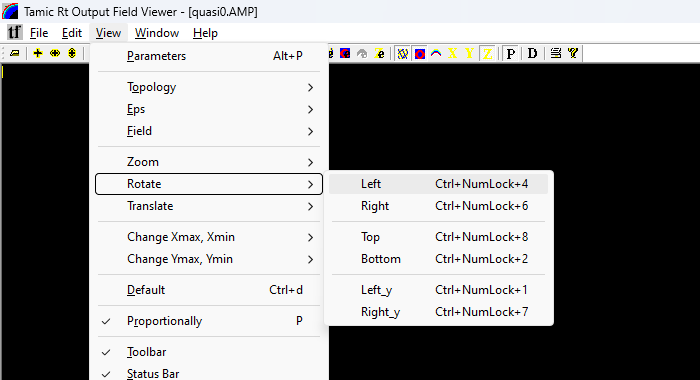
| Пункт | Клавиша | Действие |
|---|---|---|
| Left | Ctrl+NumLock+4 |
Повернуть влево. |
| Right | Ctrl+NumLock+6 |
Повернуть вправо. |
| Top | Ctrl+NumLock+8 |
Наклонить вверх. |
| Bottom | Ctrl+NumLock+2 |
Наклонить вниз. |
| Left_y | Ctrl+NumLock+1 |
Поворот вокруг оси Y влево. |
| Right_y | Ctrl+NumLock+7 |
Поворот вокруг оси Y вправо. |
5.3.6. View → Translate (сдвиг сцены)
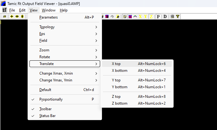
| Пункт | Клавиша | Действие |
|---|---|---|
| X top / X bottom | Alt+NumLock+6 / Alt+NumLock+4 |
Сдвиг сцены по оси X. |
| Y top / Y bottom | Alt+NumLock+7 / Alt+NumLock+1 |
Сдвиг сцены по оси Y. |
| Z top / Z bottom | Alt+NumLock+8 / Alt+NumLock+2 |
Сдвиг сцены по оси Z (приближение/отдаление). |
5.3.7. View → Change Xmax,Xmin и Change Ymax,Ymin (сдвиг окна данных)
Сдвигают видимый диапазон данных (не масштаб, а «прокрутку» по координате).
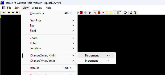
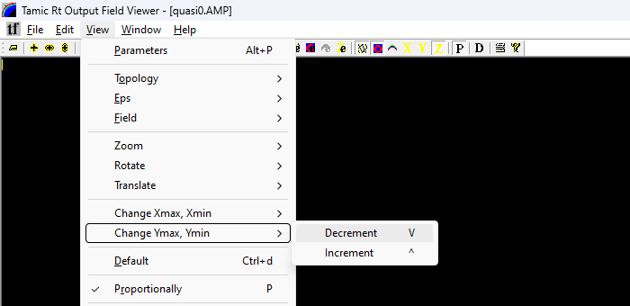
| Подменю | Пункт | Клавиша | Действие |
|---|---|---|---|
| Change Xmax, Xmin | Decrement | ← |
Сдвинуть диапазон X влево. |
| Change Xmax, Xmin | Increment | → |
Сдвинуть диапазон X вправо. |
| Change Ymax, Ymin | Decrement | V |
Сдвинуть диапазон Y вниз. |
| Change Ymax, Ymin | Increment | ^ |
Сдвинуть диапазон Y вверх. |
5.4. Window (Окно)
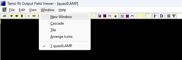
| Пункт | Перевод | Действие |
|---|---|---|
| New Window | Новое окно | Открыть ещё одно окно для того же документа. |
| Cascade | Каскадом | Расположить окна каскадом. |
| Tile | Мозаикой | Расположить окна мозаикой. |
| Arrange Icons | Упорядочить значки | Упорядочить свёрнутые окна. |
| (список 1 …) | Открытые документы | Переключение между открытыми файлами (галочка — активный). |
5.5. Help (Справка)
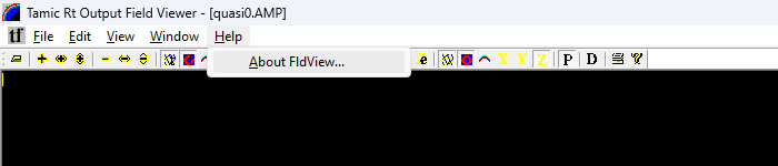
| Пункт | Перевод | Действие |
|---|---|---|
| About FldView… | О программе | Сведения о версии (раздел 6.4). |
6. Диалоговые окна
6.1. Parameters (Параметры вида)
Вызывается через View → Parameters (Alt+P). Это окно с четырьмя вкладками — Place, Topology,
Eps, Field — где собраны все настройки отображения. Внизу — кнопки OK (применить и закрыть),
Отмена (Cancel), Применить (Apply).
Вкладка Place — оси и общий вид:
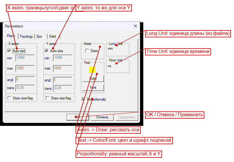
- X axies / Y axies — настройки осей X и Y:
- Auto size — автоматически подбирать границы (галочка); при снятии можно задать min и max вручную;
- angl — угол наклона оси (для 3D);
- trans — сдвиг по оси;
- Draw size flag — рисовать размерную шкалу по этой оси.
- Axies → Draw — рисовать координатные оси.
- Text → Color / Font — цвет и шрифт подписей осей (образец цвета показан квадратом).
- Long Unit / Time Unit — единицы длины и времени, прочитанные из файла (например,
mm,ns) — только для чтения. - Proportionally — сохранять одинаковый масштаб осей X и Y.
Вкладка Topology — слой топологии:
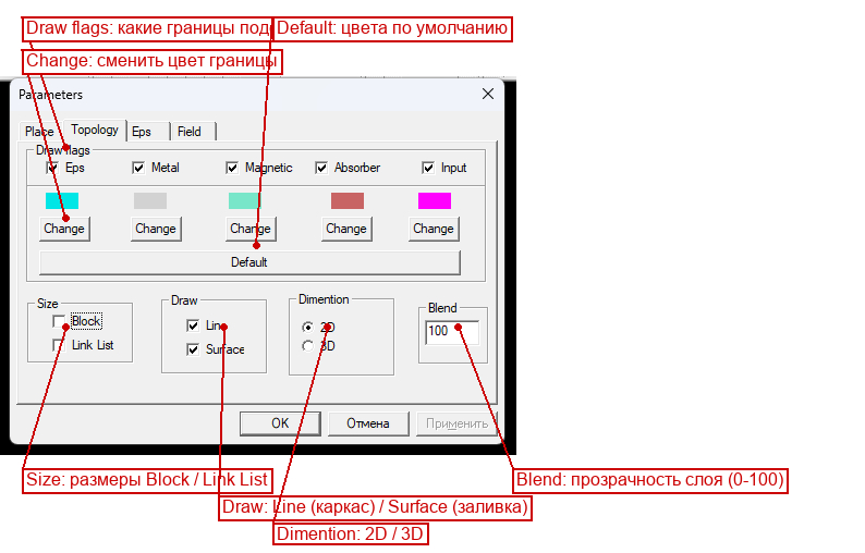
- Draw flags — какие границы подсвечивать: Eps, Metal, Magnetic, Absorber, Input; рядом образец цвета и кнопка Change (сменить цвет); кнопка Default возвращает цвета по умолчанию.
- Size — показывать размеры: Block (блоки), Link List (список связей).
- Draw — Line (каркас) и/или Surface (заливка).
- Dimention — 2D или 3D.
- Blend — степень прозрачности слоя (0–100).
Вкладка Eps — слой диэлектрической проницаемости:
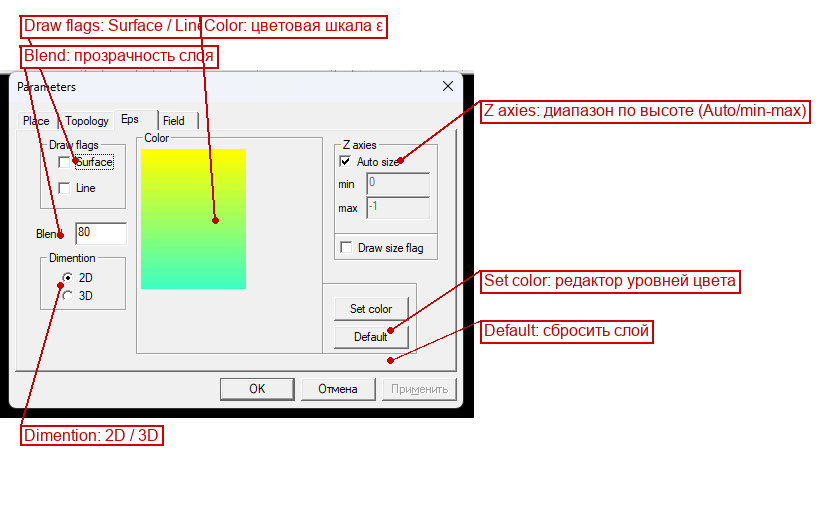
- Draw flags — Surface и/или Line.
- Color — цветовая шкала (градиент), которой раскрашивается ε.
- Blend — прозрачность слоя.
- Dimention — 2D / 3D.
- Z axies — диапазон по высоте: Auto size (авто) либо min/max вручную; Draw size flag — шкала по Z.
- Set color — открыть редактор уровней цвета (раздел 6.3).
- Default — сбросить настройки слоя.
Вкладка Field — слой поля:
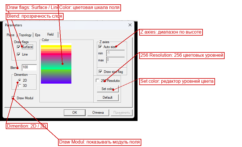
Состав тот же, что у вкладки Eps, плюс:
- 256 Resolution — использовать 256 цветовых уровней (более плавная картинка вместо 20/40 уровней).
- Draw Modul — показывать модуль поля (а не знаковое значение).
6.2. (резерв)
6.3. Auto color (Редактор уровней цвета)
Вызывается кнопкой Set color на вкладках Field/Eps окна Parameters (или View → Field → Level, Alt+E).
Позволяет вручную задать цвет каждого из уровней раскраски.
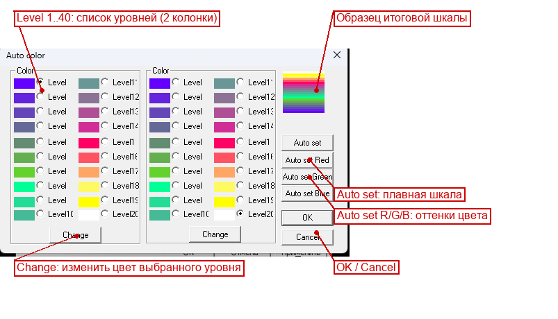
- Level 1 … Level 40 — список уровней (двумя колонками по 20); рядом — образец цвета каждого уровня; выбранный уровень отмечается переключателем.
- Change — изменить цвет выбранного уровня (открывает стандартный выбор цвета Windows).
- Auto set — автоматически построить плавную шкалу цветов.
- Auto set Red / Green / Blue — построить шкалу в оттенках красного / зелёного / синего.
- OK — применить; Cancel — отмена.
Есть также упрощённое окно «Value for color level» (показывает числовые значения, соответствующие уровням цвета) — оно открывается из режима View → Field → Value.
6.4. About (О программе)
Вызывается через Help → About FldView… или кнопкой .
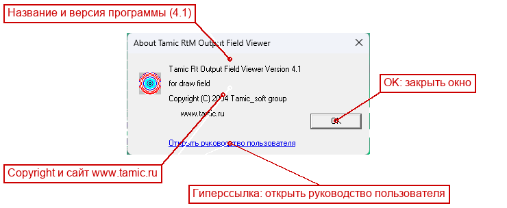
Показывает: название Tamic Rt Output Field Viewer, версию 4.1, назначение for draw field, copyright Tamic_soft group (2004) и адрес www.tamic.ru.
В нижней части окна находится синяя гиперссылка «Открыть руководство пользователя» — щелчок по ней открывает это руководство в программе по умолчанию. Кнопка OK закрывает окно.
7. Управление видом мышью и клавиатурой
- Масштаб — клавиши
+/−(иX/Y,Shift+X/Shift+Yпо отдельной оси), либо кнопки 2–7. - Прокрутка области (сдвиг видимого окна данных) — стрелки
←/→(по X) и^/V(по Y). - Поворот 3D-сцены —
Ctrl+ цифры NumLock (меню Rotate). - Сдвиг 3D-сцены / приближение —
Alt+ цифры NumLock (меню Translate). - Сброс вида —
Ctrl+D(Default) — если «потеряли» картинку, нажмите эту комбинацию. - Пропорции осей —
P(Proportionally) — чтобы круг не выглядел эллипсом.
8. Входные данные: файлы поля .tf, .AMP, .FAZ
8.1. Какие файлы открывает программа
FieldView открывает файлы распределения поля трёх расширений (фильтр в окне открытия —
FldVie Files (*.tf;*.AMP;*.FAZ;)):
| Расширение | Содержимое | Кто создаёт |
|---|---|---|
.AMP |
Амплитуда (модуль) поля на частоте анализа | счётные ядра PlanarRT_H / PlanarRT_X |
.FAZ |
Фаза поля на частоте анализа | счётные ядра PlanarRT_H / PlanarRT_X |
.tf |
Мгновенное распределение поля на конкретном шаге расчёта | счётные ядра PlanarRT_H / PlanarRT_X |
Все три файла имеют одинаковый внутренний формат (различается только смысл значений) и создаются
ядром по команде FIELD_DISTRIBUTION_M в секции #OUTPUT файла-шаблона .tpl (см. руководство по
PlanarRT_H, раздел 7). Сам пользователь эти файлы не пишет вручную — они получаются как результат
расчёта.
8.2. Внутренний формат файла
Файл состоит из текстового заголовка (11 строк, кодировка ASCII, перевод строки CR LF) и
двоичного массива значений поля.
Пример заголовка (из samples/SAMPLE_R/1/quasi0.AMP):
#TMC_GraphicsOutputFieldFile FormVer2.0 2000
#TMCGROFLD_nT 5653
#TMCGROFLD_Time 8.00008e-009
#TMCGROFLD_Delta 0.0006
#TMCGROFLD_Xmin 0
#TMCGROFLD_Ymin 0
#TMCGROFLD_Accuracy 8
#TMCGROFLD_LongUnit mm 0.001
#TMCGROFLD_TimeUnit ns 1e-009
#TMCGROFLD_nX 688
#TMCGROFLD_nY 502
Назначение строк заголовка:
| Строка | Что задаёт |
|---|---|
#TMC_GraphicsOutputFieldFile FormVer2.0 2000 |
Сигнатура формата — обязательная первая строка. По ней программа узнаёт «свой» файл. |
#TMCGROFLD_nT |
Номер временно́го шага, на котором сделан снимок (для .AMP/.FAZ обычно 0). |
#TMCGROFLD_Time |
Физическое время снимка (в системных единицах СИ — секундах). |
#TMCGROFLD_Delta |
Шаг пространственной сетки Δ. |
#TMCGROFLD_Xmin |
Координата левого края области по X. |
#TMCGROFLD_Ymin |
Координата нижнего края области по Y. |
#TMCGROFLD_Accuracy |
Размер одного числа в байтах: 4 — float (одинарная точность), 8 — double (двойная). |
#TMCGROFLD_LongUnit |
Единица длины и множитель перевода в метры (например, mm 0.001). |
#TMCGROFLD_TimeUnit |
Единица времени и множитель перевода в секунды (например, ns 1e-009). |
#TMCGROFLD_nX |
Число узлов сетки по оси X (столбцов). Должно быть ≥ 2. |
#TMCGROFLD_nY |
Число узлов сетки по оси Y (строк). Должно быть ≥ 2. |
После заголовка идёт двоичная часть: nY строк по nX чисел в каждой. Каждое число — это значение
поля в узле сетки, записанное как float (если Accuracy = 4) или double (если Accuracy = 8). Перед
каждой строкой данных стоит разделитель CR LF (два байта). Порядок обхода: сначала по X (внутренний
цикл), затем по Y (внешний).
Схематично весь файл:
[11 строк текстового заголовка, каждая оканчивается CR LF]
[CR LF][nX чисел строки Y=0][CR LF][nX чисел строки Y=1] … [CR LF][nX чисел строки Y=nY-1]
Примечания о формате. - Строки заголовка начинаются с
#— это «ключи», программа сверяет их и считывает значения. - Числовые значения в заголовке (Time,Delta, …) выводятся в формате%lg(например,8.00008e-009). - Физический размер картинки по X равенnX · Delta(в единицахLongUnit), по Y —nY · Delta. Для примера выше:688 · 0.0006 м = 0.4128 м = 412.8 мм. - Менять файл вручную не нужно и не рекомендуется — он двоичный; неверная правка приведёт к ошибкеbad data fileпри открытии. Чтобы получить другое распределение, измените расчёт в.tplи пересчитайте ядром.
8.3. Где взять примеры
Готовые файлы поля лежат в каталоге тестовых данных, например:
samples/SAMPLE_R/1/quasi0.AMP,quasi0.FAZ— амплитуда и фаза для примера из руководства PlanarRT_H;samples/SAMPLE_R/LINZA/rupor1.tf,rupor1.AMP,rupor1.FAZ— рупор с линзой;samples/SAMPLE_R/METAL/RUPOR/r7.tf,r7.AMP,r7.FAZ— металлический рупор.
9. Типовые сценарии
Посмотреть амплитуду поля (плоская картина):
1. File → Open… → выбрать файл .AMP.
2. Убедиться, что включён слой Field → Surface (кнопка 23 или S).
3. При необходимости — View → Default (Ctrl+D), затем подобрать масштаб +/−.
4. Для более плавной раскраски открыть View → Parameters → Field и включить 256 Resolution.
Перейти к трёхмерному рельефу поля:
1. Открыть файл, включить Field → Surface.
2. Нажать Field → Dimension 2/3 (кнопка 24 или D) — картинка станет объёмной.
3. Поворачивать сцену через View → Rotate (Ctrl+NumLock-цифры), приближать — View → Translate → Z.
Сравнить амплитуду и фазу:
1. Открыть .AMP.
2. Window → New Window или повторно File → Open… для .FAZ.
3. Расположить окна Window → Tile.
Настроить цветовую шкалу под свои уровни:
1. View → Parameters → Field → кнопка Set color (или View → Field → Level, Alt+E).
2. Выбрать уровень, нажать Change и задать цвет; либо Auto set для плавной шкалы.
Узнать числовое значение поля в точке:
1. View → Field → Value (Alt+A).
2. Подвести курсор к нужной точке — значение покажется в подписи/строке состояния.
10. Возможные проблемы
| Симптом | Что проверить |
|---|---|
При открытии — ошибка bad data file |
Файл должен начинаться со строки #TMC_GraphicsOutputFieldFile FormVer2.0 2000; не открывайте им посторонние файлы. |
Ошибка nX < 2 / nY < 2 |
Файл пустой или повреждён (в нём не записан массив). Пересчитайте ядром. |
Ошибка abnormal accuracy |
В заголовке Accuracy не равен 4 или 8 — файл повреждён. |
| Область отрисовки чёрная | Включите слой Field (кнопки 22–23 / S,L) и нажмите View → Default (Ctrl+D). |
| Картинка «уехала» за пределы окна | View → Default (Ctrl+D), затем View → Proportionally (P). |
| Круглые объекты выглядят овальными | Включите View → Proportionally (P). |
| 3D-картинку не видно после поворота | Ctrl+D (сброс), затем поворачивайте небольшими шагами. |
| Поворот/сдвиг с NumLock не работает | Убедитесь, что включён NumLock на клавиатуре. |
11. Связанные программы и документы
- PlanarRT_H / PlanarRT_X — счётные ядра, создающие файлы поля
.tf/.AMP/.FAZ. См.planar_rt_h.md,planar_rt_x.md. - TMCROS — просмотр временно́го сигнала (
.t). См.tmcros.md. - TMCGROUT — просмотр S-матрицы (
.s). См.tmcgrout.md. - TMC_DN — просмотр диаграммы направленности. См.
tmc_dn.md. - Формат данных поля задаётся библиотекой TMCIndan (модуль
FieldIntegrated) — см.docs/api/libs/tmcindan.md.
User manual — FieldView (FieldView.exe)
Program: Tamic Rt Output Field Viewer (internal project name FldView, the executable
FieldView.exe, version 4.1). The program's interface is in English — the manual gives the English item names as in the program, with an explanation next to them. The captions on the screenshots are in Russian.
1. Purpose of the program
FieldView is the field-distribution viewer of the TMC Suite package. The compute kernels PlanarRT_H and PlanarRT_X save "maps" of the field in the computation area during the electrodynamic computation, and FieldView draws these maps as two-dimensional color pictures or three-dimensional surfaces (using OpenGL).
In simple terms: the kernel computed how the field is distributed over the plane of the model and wrote it to a file; FieldView opens such a file and shows it as a picture — where the field is stronger, where weaker, how it is organized inside a horn, a lens, a resonator, etc.
The program can show three independent "layers" of the same area, each with its own color and rendering settings:
| Layer | What it shows |
|---|---|
| Field | the main field distribution from the open file; |
| Eps (ε) | the distribution of the medium's permittivity; |
| Topology | the model geometry and its boundaries (metal, absorber, dielectric, input, magnetic wall). |
This is an MDI program: several field files can be opened in one window and compared (the Window menu).
2. Launching the program and opening data
- Launch the file
FieldView.exe(folderdist/win32/bin/ordist/win64/bin/). The main window opens. - Open a field file: menu File → Open… (or the
button on the toolbar, or
Ctrl+O). - In the file-selection dialog choose a file of one of the supported types —
.tf,.AMPor.FAZ(for example,samples/SAMPLE_R/1/quasi0.AMP). Details on the formats are in section 8. - After opening, the file name appears in the window title:
Tamic Rt Output Field
   Viewer - [quasi0.AMP]
. - The field is drawn in the work area. If the image is not visible — check whether
the Field layer is enabled (buttons 22–23 on the toolbar or menu View →
Field) and press View → Default (
Ctrl+D) to restore the standard scale and position.
You can launch the program with a file at once: drag the
.AMP/.FAZ/.tfonto the program icon or pass the path as a command-line argument:FieldView.exe "path\to\file.AMP".
3. The main window
The main window consists of five zones (shown with numbers in the figure in section 1):
| # | Zone | Purpose |
|---|---|---|
| 1 | Title bar | The program name and the name of the open file. |
| 2 | Menu bar | All commands: File, Edit, View, Window, Help. |
| 3 | Toolbar | Quick-access buttons for the most frequent commands (35 buttons). |
| 4 | Rendering area | Here OpenGL draws the field / topology / ε distribution. Controlled with the mouse and keys (scale, rotate, shift). |
| 5 | Status bar | On the left — service messages and the current view boundaries (Xmin/Xmax, Ymin/Ymax, Delta); on the right — the parameters of the open file (nT — step number, t — time). |
About the rendering-area screenshots. Some of the overview pictures in this manual were made in an environment where the contents of the OpenGL window are not captured by a screenshot, so the rendering area (zone 4) looks black in them. On a real computer a color field picture is displayed here (examples of a "live" result —
main-window-field.png,field-3d.png,eps-layer.png).
4. The toolbar
The toolbar duplicates the most useful commands. The buttons from left to right are numbered 1–35 and grouped (the groups are separated by vertical gaps):
| # | Button | Command | Shortcut | What it does |
|---|---|---|---|---|
| 1 | |
File → Open | Ctrl+O |
Open a field file (.tf/.AMP/.FAZ/.ex). |
| 2 | |
Zoom + | + |
Zoom in (both axes). |
| 3 | |
Zoom +X | X |
Zoom in only on the X axis. |
| 4 | |
Zoom +Y | Y |
Zoom in only on the Y axis. |
| 5 | |
Zoom − | − |
Zoom out (both axes). |
| 6 | |
Zoom −X | Shift+X |
Zoom out on the X axis. |
| 7 | |
Zoom −Y | Shift+Y |
Zoom out on the Y axis. |
| 8 | |
Topology → Line | Shift+L |
Topology layer: draw with lines (wireframe). |
| 9 | |
Topology → Surface | Shift+S |
Topology layer: draw as a filled surface. |
| 10 | |
Topology → Dimension 2/3 | Shift+D |
Switch the topology between 2D and 3D. |
| 11 | |
Boundary → Eps | E |
Highlight the dielectric (ε) boundaries. |
| 12 | |
Boundary → Metal | M |
Highlight the metal boundaries. |
| 13 | |
Boundary → Magnetic | N |
Highlight the magnetic-wall boundaries. |
| 14 | |
Boundary → Absorber | A |
Highlight the absorber boundaries. |
| 15 | |
Boundary → Input | I |
Highlight the input (port) boundaries. |
| 16 | |
Topology → Dimensions → Block | K |
Show block dimensions/numbering. |
| 17 | |
Topology → Dimensions → Link_List | Alt+K |
Show dimensions by the link list (Link List). |
| 18 | |
Eps → Line | Alt+L |
ε layer: draw with lines. |
| 19 | |
Eps → Surface | Alt+S |
ε layer: draw as a filled surface. |
| 20 | |
Eps → Dimension 2/3 | Alt+D |
Switch ε between 2D and 3D. |
| 21 | |
Eps → Size | Alt+J |
Auto-size the ε layer along the Z axis (height). |
| 22 | |
View → Eps → Type → Eps+ | — | Quantity mode: show the permittivity ε (the normal mode, always available). |
| 23 | |
View → Eps → Type → N | — | Plasma (X-mode): show the electron concentration N. Available only if the data contains plasma (RECT_STAT_N blocks). |
| 24 | |
View → Eps → Type → B | — | Plasma (X-mode): show the external magnetic field B (magnetization). Available if there are RECT_STAT_B blocks. |
| 25 | |
View → Eps → Type → Y | — | Plasma (X-mode): show the losses Y. Available if there are RECT_STAT_Y blocks. |
| 26 | |
Field → Line | L |
Field layer: draw with lines. |
| 27 | |
Field → Surface | S |
Field layer: draw as a filled surface. |
| 28 | |
Field → Dimension 2/3 | D |
Switch the field between 2D and 3D. |
| 29 | |
Size → along an X axies | Ctrl+J |
Show the dimension grid along the X axis. |
| 30 | |
Size → along an Y axies | Shift+J |
Show the dimension grid along the Y axis. |
| 31 | |
Field → Size | J |
Auto-size the field layer along the Z axis (relief height). |
| 32 | |
View → Proportionally | P |
Toggle proportional scaling of the X and Y axes. |
| 33 | |
View → Default | Ctrl+D |
Reset the view to the standard parameters. |
| 34 | |
File → Print | Ctrl+P |
Print the current image. |
| 35 | |
Help → About | — | About the program (version). |
Buttons 22–25 (EPS · N · B · Y) are new. This is a switch of the displayed quantity for plasma computations (X-mode,
tmc_rtx): E (yellow) — the permittivity ε; N (red) — the electron concentration; B (blue) — the magnetization magnetic field; Y (green) — the losses. The N, B, Y buttons are active (colored) only when the open field contains the corresponding plasma; otherwise they are gray (inactive). Details in section 5.3.2.1.Tip: hovering the cursor over a button in the program shows its English name as a tooltip, and a short description appears in the status bar.
A clean view of the toolbar without numbering:
5. The menus
5.1. File
| Item | Translation | Shortcut | Action |
|---|---|---|---|
| New | Create | Ctrl+N |
A new empty document. |
| Open… | Open | Ctrl+O |
Open a field file (.tf/.AMP/.FAZ). |
| Close | Close | — | Close the current document. |
| Save | Save | Ctrl+S |
Save the document. |
| Save As… | Save as | — | Save under a different name. |
| Print… | Ctrl+P |
Print the image. | |
| Print Preview | Print preview | — | Preview before printing. |
| Print Setup… | Print settings | — | Choose the printer and page parameters. |
| (list 1, 2, 3…) | Recent files | — | Quick opening of recently used files. |
| Exit | Exit | — | Close the program. |
5.2. Edit
| Item | Translation | Shortcut | Action |
|---|---|---|---|
| Undo | Undo | Ctrl+Z |
A standard command (unavailable in the current mode — gray). |
| Cut / Copy / Paste | Cut / Copy / Paste | Ctrl+X / Ctrl+C / Ctrl+V |
Clipboard commands (unavailable — gray). |
In this version the Edit menu is not used: the program only views the data, it does not edit it.
5.3. View
The main display-control menu. It contains the parameters-window command, three layer submenus (Topology / Eps / Field), the view-control submenus (Zoom / Rotate / Translate), and toggles.
| Item | Translation | Shortcut | Action |
|---|---|---|---|
| Parameters | Parameters | Alt+P |
Open the view-settings window (section 6.1). |
| Topology ► | Topology | — | Topology-layer submenu (5.3.1). |
| Eps ► | Dielectric ε | — | ε-layer submenu (5.3.2). |
| Field ► | Field | — | Field-layer submenu (5.3.3). |
| Zoom ► | Zoom | — | Zoom submenu (5.3.4). |
| Rotate ► | Rotate | — | Rotation submenu (3D) (5.3.5). |
| Translate ► | Translate | — | Scene-shift submenu (5.3.6). |
| Change Xmax, Xmin ► | Shift window along X | — | Shift the visible X range (5.3.7). |
| Change Ymax, Ymin ► | Shift window along Y | — | Shift the visible Y range (5.3.7). |
| Default | Default | Ctrl+d |
Reset the view to the standard parameters. |
| Proportionally | Proportionally | P |
Keep the same scale for the X and Y axes (a check mark = on). |
| Toolbar | Toolbar | — | Show/hide the toolbar. |
| Status Bar | Status bar | — | Show/hide the status bar. |
5.3.1. View → Topology (the topology layer)
| Item | Shortcut | Action |
|---|---|---|
| Line | Shift+L |
Draw the topology with lines (wireframe). |
| Surface | Shift+S |
Draw the topology as a filled surface. |
| Dimension 2/3 | Shift+D |
Switch 2D 3D. |
| Size ► | — | The dimension grid along the axes (5.3.1.1). |
| Dimensions ► | — | Show block dimensions / the link list (5.3.1.2). |
| Boundary ► | — | Highlight material boundaries (5.3.1.3). |
5.3.1.1. Topology → Size — the dimension grid:
- along an X axies (
Ctrl+J) — put dimensions along the X axis; - along an Y axies (
Shift+J) — put dimensions along the Y axis.
5.3.1.2. Topology → Dimensions — showing element dimensions:
- Block (
K) — block dimensions/numbering; - Link_List (
Alt+K) — dimensions by the link list (Link List).
5.3.1.3. Topology → Boundary — highlighting material boundaries (a check mark = the layer is on):
- Eps (
E) — dielectric boundaries; - Metal (
M) — metal boundaries; - Magnetic (
N) — magnetic-wall boundaries; - Absorber (
A) — absorber boundaries; - Input (
I) — input (excitation port) boundaries.
5.3.2. View → Eps (the dielectric layer)
| Item | Shortcut | Action |
|---|---|---|
| Line | Alt+L |
Draw ε with lines. |
| Surface | Alt+S |
Draw ε as a filled surface. |
| Dimension 2/3 | Alt+D |
Switch 2D 3D (may be gray in the current version). |
| Size | Alt+J |
Auto-size the ε layer along the Z axis. |
| Type ► | — | Choose the displayed quantity: ε / N / B / Y (plasma). See 5.3.2.1. |
5.3.2.1. View → Eps → Type — the displayed quantity (X-mode plasma)
The Type submenu (and the new toolbar buttons 22–25) choose which physical
quantity to draw in the "Eps" layer for plasma computations in the X-mode (the
tmc_rtx kernel):
| Menu item | Button | Quantity | When available |
|---|---|---|---|
| Eps+ | — E, yellow |
Permittivity ε (the normal mode) | Always |
| N | — N, red |
Plasma electron concentration N, m⁻³ | Only if the field has RECT_STAT_N blocks |
| B | — B, blue |
External magnetization magnetic field B, T | Only if there are RECT_STAT_B blocks |
| Y | — Y, green |
Plasma losses Y | Only if there are RECT_STAT_Y blocks |
How to use it. Open a field computed by the X kernel with plasma (a .ex/.tf
file next to the topology .tt, where the RECT_STAT_N/_B/_Y blocks are set), then
press the desired button (or menu item). The "Eps" layer switches from the ordinary
ε to the chosen quantity. If there is no plasma in the data, the N/B/Y buttons are
gray (inactive) — only Eps+ is available. The chosen mode is remembered
between runs.
The N, B, Y quantities correspond to the
RECT_STAT_Nblocks (electron concentration, m⁻³),RECT_STAT_B(magnetization magnetic field, T) andRECT_STAT_Y(losses) in the.tpltask template — see the PlanarRT_X kernel manual.
5.3.3. View → Field (the field layer)
| Item | Shortcut | Action |
|---|---|---|
| Line | L |
Draw the field with lines. |
| Surface | S |
Draw the field as a filled surface. |
| Dimension 2/3 | D |
Switch 2D 3D. |
| Size | J |
Auto-size the field layer along the Z axis (relief height). |
| Level | Alt+E |
Open the color levels window (section 6.3). |
| Value | Alt+A |
The mode showing the numeric value of the field under the cursor. |
| Modul | Alt+M |
Show the magnitude of the field. |
5.3.4. View → Zoom
| Item | Shortcut | Action |
|---|---|---|
| Zoom + | + |
Zoom in (both axes). |
| Zoom +X | X |
Zoom in on X. |
| Zoom +Y | Y |
Zoom in on Y. |
| Zoom − | − |
Zoom out (both axes). |
| Zoom −X | Shift+X |
Zoom out on X. |
| Zoom −Y | Shift+Y |
Zoom out on Y. |
5.3.5. View → Rotate (rotation, for 3D)
| Item | Shortcut | Action |
|---|---|---|
| Left | Ctrl+NumLock+4 |
Rotate left. |
| Right | Ctrl+NumLock+6 |
Rotate right. |
| Top | Ctrl+NumLock+8 |
Tilt up. |
| Bottom | Ctrl+NumLock+2 |
Tilt down. |
| Left_y | Ctrl+NumLock+1 |
Rotate around the Y axis to the left. |
| Right_y | Ctrl+NumLock+7 |
Rotate around the Y axis to the right. |
5.3.6. View → Translate (scene shift)
| Item | Shortcut | Action |
|---|---|---|
| X top / X bottom | Alt+NumLock+6 / Alt+NumLock+4 |
Shift the scene along the X axis. |
| Y top / Y bottom | Alt+NumLock+7 / Alt+NumLock+1 |
Shift the scene along the Y axis. |
| Z top / Z bottom | Alt+NumLock+8 / Alt+NumLock+2 |
Shift the scene along the Z axis (zoom in/out). |
5.3.7. View → Change Xmax,Xmin and Change Ymax,Ymin (data-window shift)
They shift the visible data range (not the scale, but "scrolling" along the coordinate).
| Submenu | Item | Shortcut | Action |
|---|---|---|---|
| Change Xmax, Xmin | Decrement | ← |
Shift the X range left. |
| Change Xmax, Xmin | Increment | → |
Shift the X range right. |
| Change Ymax, Ymin | Decrement | V |
Shift the Y range down. |
| Change Ymax, Ymin | Increment | ^ |
Shift the Y range up. |
5.4. Window
| Item | Translation | Action |
|---|---|---|
| New Window | New window | Open another window for the same document. |
| Cascade | Cascade | Arrange the windows in a cascade. |
| Tile | Tile | Arrange the windows tiled. |
| Arrange Icons | Arrange icons | Arrange the minimized windows. |
| (list 1 …) | Open documents | Switch between the open files (a check mark — the active one). |
5.5. Help
| Item | Translation | Action |
|---|---|---|
| About FldView… | About | Version information (section 6.4). |
6. Dialog windows
6.1. Parameters (view parameters)
Invoked via View → Parameters (Alt+P). This is a window with four tabs —
Place, Topology, Eps, Field — where all the display settings are
collected. At the bottom are the OK (apply and close), Cancel, and
Apply buttons.
The Place tab — axes and general view:
- X axies / Y axies — settings for the X and Y axes:
- Auto size — automatically fit the boundaries (a check mark); when unchecked, you can set min and max manually;
- angl — the tilt angle of the axis (for 3D);
- trans — the shift along the axis;
- Draw size flag — draw the dimension scale along this axis.
- Axies → Draw — draw the coordinate axes.
- Text → Color / Font — the color and font of the axis labels (a color sample is shown as a square).
- Long Unit / Time Unit — the length and time units read from the file (for
example,
mm,ns) — read-only. - Proportionally — keep the same scale for the X and Y axes.
The Topology tab — the topology layer:
- Draw flags — which boundaries to highlight: Eps, Metal, Magnetic, Absorber, Input; next to each is a color sample and a Change button (change the color); the Default button restores the default colors.
- Size — show dimensions: Block (blocks), Link List (the link list).
- Draw — Line (wireframe) and/or Surface (fill).
- Dimention — 2D or 3D.
- Blend — the transparency degree of the layer (0–100).
The Eps tab — the permittivity layer:
- Draw flags — Surface and/or Line.
- Color — the color scale (gradient) used to color ε.
- Blend — the layer transparency.
- Dimention — 2D / 3D.
- Z axies — the height range: Auto size (auto) or min/max manually; Draw size flag — the Z scale.
- Set color — open the color-levels editor (section 6.3).
- Default — reset the layer settings.
The Field tab — the field layer:
The contents are the same as the Eps tab, plus:
- 256 Resolution — use 256 color levels (a smoother picture instead of 20/40 levels).
- Draw Modul — show the magnitude of the field (rather than the signed value).
6.2. (reserved)
6.3. Auto color (the color-levels editor)
Invoked with the Set color button on the Field/Eps tabs of the
Parameters window (or View → Field → Level, Alt+E). It lets you manually set
the color of each of the coloring levels.
- Level 1 … Level 40 — the list of levels (in two columns of 20); next to each is a color sample of the level; the selected level is marked with a radio button.
- Change — change the color of the selected level (opens the standard Windows color selector).
- Auto set — automatically build a smooth color scale.
- Auto set Red / Green / Blue — build a scale in shades of red / green / blue.
- OK — apply; Cancel — cancel.
There is also a simplified "Value for color level" window (it shows the numeric values corresponding to the color levels) — it opens from the View → Field → Value mode.
6.4. About
Invoked via Help → About FldView… or the
button.
Shows: the name Tamic Rt Output Field Viewer, version 4.1, the purpose for draw field, the copyright Tamic_soft group (2004) and the address www.tamic.ru.
At the bottom of the window there is a blue "Open user manual" hyperlink — clicking it opens this manual in the default program. The OK button closes the window.
7. Controlling the view with the mouse and keyboard
- Scale — the
+/−keys (andX/Y,Shift+X/Shift+Yfor a single axis), or buttons 2–7. - Scrolling the area (shifting the visible data window) — the arrows
←/→(along X) and^/V(along Y). - Rotating the 3D scene —
Ctrl+ NumLock digits (the Rotate menu). - Shifting the 3D scene / zooming —
Alt+ NumLock digits (the Translate menu). - Resetting the view —
Ctrl+D(Default) — if you "lost" the picture, press this combination. - Axis proportions —
P(Proportionally) — so that a circle does not look like an ellipse.
8. Input data: the field files .tf, .AMP, .FAZ
8.1. Which files the program opens
FieldView opens field-distribution files of three extensions (the filter in the
open dialog is FldVie Files (*.tf;*.AMP;*.FAZ;)):
| Extension | Contents | Who creates it |
|---|---|---|
.AMP |
The amplitude (magnitude) of the field at the analysis frequency | the PlanarRT_H / PlanarRT_X kernels |
.FAZ |
The phase of the field at the analysis frequency | the PlanarRT_H / PlanarRT_X kernels |
.tf |
The instantaneous field distribution at a specific computation step | the PlanarRT_H / PlanarRT_X kernels |
All three files have the same internal format (only the meaning of the values
differs) and are created by the kernel with the FIELD_DISTRIBUTION_M command in
the #OUTPUT section of the .tpl template file (see the PlanarRT_H manual,
section 7). The user does not write these files by hand — they are obtained as
the result of a computation.
8.2. The internal file format
The file consists of a text header (11 lines, ASCII encoding, line break CR
LF) and a binary array of field values.
An example header (from samples/SAMPLE_R/1/quasi0.AMP):
#TMC_GraphicsOutputFieldFile FormVer2.0 2000
#TMCGROFLD_nT 5653
#TMCGROFLD_Time 8.00008e-009
#TMCGROFLD_Delta 0.0006
#TMCGROFLD_Xmin 0
#TMCGROFLD_Ymin 0
#TMCGROFLD_Accuracy 8
#TMCGROFLD_LongUnit mm 0.001
#TMCGROFLD_TimeUnit ns 1e-009
#TMCGROFLD_nX 688
#TMCGROFLD_nY 502
The purpose of the header lines:
| Line | What it sets |
|---|---|
#TMC_GraphicsOutputFieldFile FormVer2.0 2000 |
The format signature — the mandatory first line. The program recognizes "its" file by it. |
#TMCGROFLD_nT |
The number of the time step at which the snapshot was made (for .AMP/.FAZ usually 0). |
#TMCGROFLD_Time |
The physical time of the snapshot (in SI units — seconds). |
#TMCGROFLD_Delta |
The spatial grid step Δ. |
#TMCGROFLD_Xmin |
The X coordinate of the left edge of the area. |
#TMCGROFLD_Ymin |
The Y coordinate of the bottom edge of the area. |
#TMCGROFLD_Accuracy |
The size of one number in bytes: 4 — float (single precision), 8 — double (double precision). |
#TMCGROFLD_LongUnit |
The length unit and the factor for converting to meters (for example, mm 0.001). |
#TMCGROFLD_TimeUnit |
The time unit and the factor for converting to seconds (for example, ns 1e-009). |
#TMCGROFLD_nX |
The number of grid nodes along the X axis (columns). Must be ≥ 2. |
#TMCGROFLD_nY |
The number of grid nodes along the Y axis (rows). Must be ≥ 2. |
After the header comes the binary part: nY rows of nX numbers each. Each
number is the field value at a grid node, written as a float (if Accuracy = 4)
or a double (if Accuracy = 8). Before each data row there is a CR LF
separator (two bytes). The traversal order: first along X (the inner loop), then
along Y (the outer loop).
The whole file schematically:
[11 lines of text header, each ending with CR LF]
[CR LF][nX numbers of row Y=0][CR LF][nX numbers of row Y=1] … [CR LF][nX numbers of row Y=nY-1]
Notes on the format. - The header lines start with
#— these are "keys"; the program checks them and reads the values. - The numeric values in the header (Time,Delta, …) are printed in the%lgformat (for example,8.00008e-009). - The physical size of the picture along X equalsnX · Delta(inLongUnitunits), along Y —nY · Delta. For the example above:688 · 0.0006 m = 0.4128 m = 412.8 mm. - You do not need and should not change the file by hand — it is binary; an incorrect edit will lead to abad data fileerror on opening. To get a different distribution, change the computation in the.tpland recompute with the kernel.
8.3. Where to get examples
Ready-made field files are in the test-data directory, for example:
samples/SAMPLE_R/1/quasi0.AMP,quasi0.FAZ— the amplitude and phase for the example from the PlanarRT_H manual;samples/SAMPLE_R/LINZA/rupor1.tf,rupor1.AMP,rupor1.FAZ— a horn with a lens;samples/SAMPLE_R/METAL/RUPOR/r7.tf,r7.AMP,r7.FAZ— a metal horn.
9. Typical scenarios
View the field amplitude (a flat picture):
1. File → Open… → select an .AMP file.
2. Make sure the Field → Surface layer is on (button 23 or S).
3. If needed — View → Default (Ctrl+D), then adjust the scale with +/−.
4. For a smoother coloring, open View → Parameters → Field and enable 256
Resolution.
Switch to the three-dimensional field relief:
1. Open a file, enable Field → Surface.
2. Press Field → Dimension 2/3 (button 24 or D) — the picture becomes 3D.
3. Rotate the scene via View → Rotate (Ctrl+NumLock digits), zoom in with
View → Translate → Z.
Compare the amplitude and the phase:
1. Open .AMP.
2. Window → New Window or File → Open… again for the .FAZ.
3. Arrange the windows with Window → Tile.
Configure the color scale for your levels:
1. View → Parameters → Field → the Set color button (or View → Field →
Level, Alt+E).
2. Select a level, press Change and set the color; or Auto set for a smooth
scale.
Find the numeric field value at a point:
1. View → Field → Value (Alt+A).
2. Bring the cursor to the desired point — the value is shown in the caption/status
bar.
10. Possible problems
| Symptom | What to check |
|---|---|
On opening — a bad data file error |
The file must start with the line #TMC_GraphicsOutputFieldFile FormVer2.0 2000; do not open foreign files with it. |
A nX < 2 / nY < 2 error |
The file is empty or corrupted (no array is written in it). Recompute with the kernel. |
An abnormal accuracy error |
In the header Accuracy is not equal to 4 or 8 — the file is corrupted. |
| The rendering area is black | Enable the Field layer (buttons 22–23 / S,L) and press View → Default (Ctrl+D). |
| The picture has "run off" beyond the window | View → Default (Ctrl+D), then View → Proportionally (P). |
| Round objects look oval | Enable View → Proportionally (P). |
| The 3D picture is not visible after rotation | Ctrl+D (reset), then rotate in small steps. |
| Rotation/shift with NumLock does not work | Make sure NumLock is on. |
11. Related programs and documents
- PlanarRT_H / PlanarRT_X — the compute kernels that create the field files
.tf/.AMP/.FAZ. Seeplanar_rt_h.md,planar_rt_x.md. - TMCROS — viewing the time signal (
.t). Seetmcros.md. - TMCGROUT — viewing the S-matrix (
.s). Seetmcgrout.md. - TMC_DN — viewing the radiation pattern. See
tmc_dn.md. - The field-data format is defined by the TMCIndan library (the
FieldIntegratedmodule) — seedocs/api/libs/tmcindan.md.