Руководство пользователя — программа TMC_DN (TMC_DN.exe)
Пакет TMC Suite. Это руководство написано простым языком и рассчитано на пользователя, который видит программу впервые. Все названия пунктов меню и кнопок приведены так, как они выглядят в программе (интерфейс — английский), а рядом дан перевод и пояснение.
1. Назначение программы
TMC_DN (исполняемый файл TMC_DN.exe, полное название — Tamic Directional Pattern Viewer, «просмотрщик диаграмм направленности Tamic») — это программа для расчёта и просмотра диаграмм направленности (ДН) антенн и антенных решёток. Проще говоря, она строит график, у которого:
- по горизонтальной оси (X) отложен угол (в радианах, в диапазоне примерно от −π до +π) — то есть направление в пространстве, куда «смотрит» антенна;
- по вертикальной оси (Y) отложен уровень диаграммы направленности (Pattern) — насколько сильно антенна излучает (или принимает) в данном направлении.
Диаграмма направленности — это «карта» того, как антенна распределяет излучение по углам: в каких направлениях она излучает сильно (главный лепесток), а в каких слабо (боковые лепестки и провалы). Для антенной решётки (множества излучателей, расставленных в пространстве) форма ДН зависит от координат элементов, их амплитуд и фаз. TMC_DN берёт описание такой решётки, рассчитывает её диаграмму направленности и рисует её в виде наглядного графика.
Что умеет программа:
- открывать готовые документы-диаграммы (файлы
.dop) или напрямую файлы описания решётки (.DAT); - рассчитывать диаграмму направленности антенной решётки по описанию её излучателей (когерентное суммирование полей всех элементов по углу);
- вычислять и показывать интегральные характеристики антенны: КНД (
Knd, в том числе в децибелах), КИП (Kip), а для крупных решёток — излучённую мощность (Emitted Power); - показывать сразу несколько диаграмм на одном поле (например, ДН разных решёток для сравнения);
- менять масштаб (увеличение/уменьшение, автоподбор по осям), сдвигать видимую область;
- настраивать цвета фона, сетки, осей и самих кривых, а также шрифт подписей;
- вносить случайные отклонения (девиации) в параметры излучателей — координаты, амплитуды, фазы — и смотреть, как при этом «портится» диаграмма; сравнивать получившуюся ДН с требуемой (эталонной) ДН;
- печатать диаграмму и сохранять настройки оформления в самом документе
.dop.
Расчёт большой решётки может занять заметное время, поэтому TMC_DN считает диаграмму в фоне и показывает окно прогресса с двумя индикаторами (готовность текущей ДН и готовность по всем ДН документа). Подробнее — раздел 6.
Чем TMC_DN отличается от «соседних» программ пакета? TMCGROUT показывает частотные характеристики (S-матрицу в зависимости от частоты), TMCROS — временны́е сигналы, а TMC_DN — диаграммы направленности (уровень излучения в зависимости от угла). Внешне все три очень похожи (сделаны по одной схеме), поэтому меню и панель инструментов у них почти одинаковые. Но TMC_DN дополнительно умеет рассчитывать ДН решётки, считать КНД/КИП и моделировать девиации — этого в других вьюверах нет.
2. Запуск и открытие данных
Как запустить программу
- Найдите файл
TMC_DN.exe(после сборки он лежит в каталогеdist/win32/binилиdist/win64/bin). - Запустите его двойным щелчком.
- При первом запуске программа разворачивается на весь экран. Если ранее уже открывались какие-либо файлы, TMC_DN попытается автоматически открыть последний из них (список «недавних файлов» хранится в реестре Windows в разделе
TMC_DN).
Какой файл открывать
TMC_DN работает с двумя основными типами файлов (подробно — в разделе 7):
| Файл | Что это | Когда открывать |
|---|---|---|
.dop |
Документ TMC_DN: текстовый файл с настройками диаграммы и ссылкой на файл(ы) описания решётки | Обычный способ. Сохраняет цвета, масштаб, список диаграмм |
.DAT |
Файл описания антенной решётки (частота, излучатели, выражение ДН элемента) | Если хотите построить диаграмму по «сырому» описанию. Программа сама создаст для него документ |
Чтобы открыть файл:
- Меню File → Open… (Файл → Открыть), либо нажмите кнопку «Открыть» на панели инструментов, либо клавиши Ctrl+O.
- В диалоге выберите нужный
.dopили.DATфайл. - Программа рассчитает диаграмму направленности (для большой решётки появится окно прогресса) и построит график.
Если вы открываете
.DAT-файл, рядом с ним будет создан документ (он хранит настройки отображения). В дальнейшем удобнее открывать именно документ.dop.
3. Главное окно
Главное окно — это многодокументное окно (MDI): внутри него могут быть открыты сразу несколько окон с разными диаграммами.
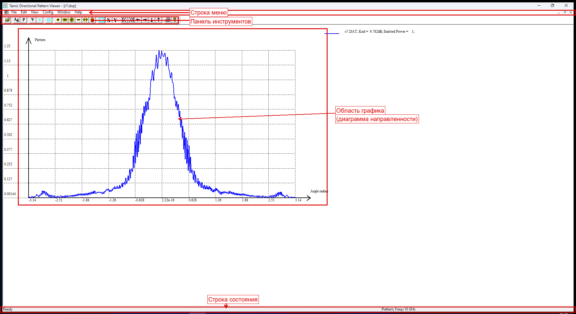
Окно состоит из четырёх зон:
- Строка меню (вверху) — все команды программы, сгруппированные по разделам (File, Edit, View, Config, Window, Help). Подробно — раздел 5.
- Панель инструментов (тулбар) — ряд кнопок-значков для самых частых действий. Подробно — раздел 4.
- Область графика (центр) — здесь рисуются оси, координатная сетка и сама диаграмма направленности. По горизонтали отложен угол (радианы), по вертикали — уровень ДН. По этой области работает мышь: можно выделить прямоугольник для увеличения (zoom), а двойной щелчок подгоняет масштаб.
- Строка состояния (статусбар) (внизу) — две панели:
- левая — координаты точки под курсором мыши (значение угла по X и значение уровня ДН по Y);
- правая — интегральные характеристики текущей диаграммы: КНД (
Knd, в том числе в дБ) и КИП (Kip), а для крупной решётки — излучённая мощность (Emitted Power) вместо КИП.
4. Панель инструментов
Панель инструментов дублирует самые частые команды меню в виде кнопок. Если панель не видна, включите её через View → Toolbar. Панель и меню у TMC_DN общие с TMCGROUT — у программы расчёта ДН (модуль DiaNapGr) собственного файла ресурсов нет, поэтому набор кнопок такой же.
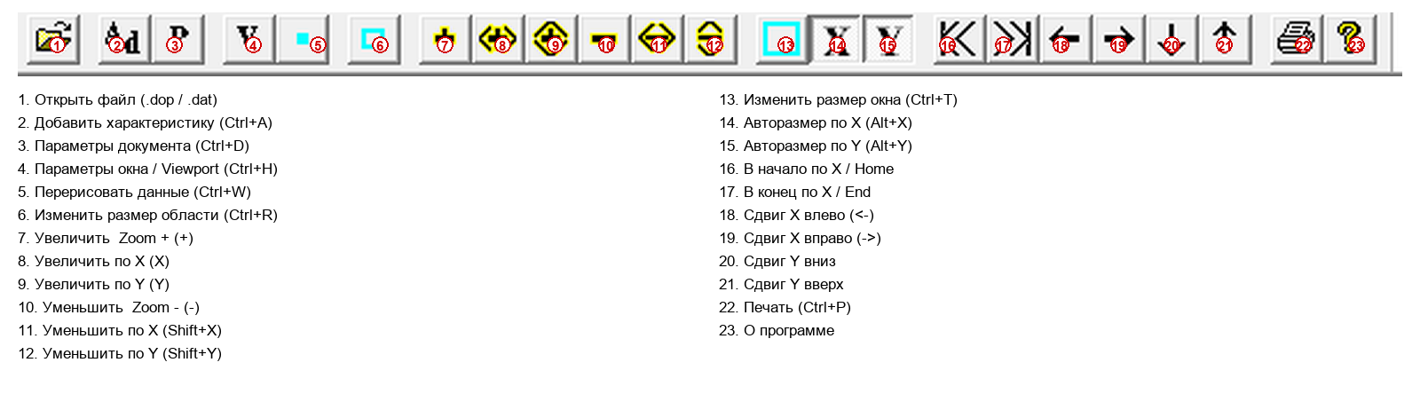
Кнопки идут слева направо. Ниже — назначение каждой.
| № | Кнопка | Название (англ./рус.) | Горячая клавиша | Что делает |
|---|---|---|---|---|
| 1 |  |
Open / Открыть файл | Ctrl+O | Открывает файл .dop или .DAT (то же, что File → Open) |
| 2 |  |
Add characteristics / Добавить характеристику | Ctrl+A | Добавляет в документ ещё одну диаграмму из выбранного .DAT-файла |
| 3 |  |
Characteristics / Параметры документа | Ctrl+D | Открывает таблицу-список всех диаграмм документа (имена, файлы, флаги показа); отсюда же доступны функции девиаций — см. раздел 6 |
| 4 |  |
Viewport / Параметры окна | Ctrl+H | Открывает диалог настройки отображения: пределы по осям, авто-масштаб, формат подписей, точки |
| 5 |  |
Redraw data / Перечитать и перерисовать | Ctrl+W | Заново читает данные и пересчитывает/перерисовывает диаграмму |
| 6 |  |
Resize viewport / Подогнать область графика | Ctrl+R | Подгоняет область рисования под размер окна |
| 7 |  |
Zoom + / Увеличить | — | Увеличивает масштаб по обеим осям |
| 8 |  |
Zoom +X / Увеличить по X | — | Увеличивает масштаб только по горизонтали (углу) |
| 9 |  |
Zoom +Y / Увеличить по Y | — | Увеличивает масштаб только по вертикали (уровню) |
| 10 |  |
Zoom − / Уменьшить | — | Уменьшает масштаб по обеим осям |
| 11 |  |
Zoom −X / Уменьшить по X | Shift+X | Уменьшает масштаб по горизонтали |
| 12 |  |
Zoom −Y / Уменьшить по Y | Shift+Y | Уменьшает масштаб по вертикали |
| 13 |  |
Resize window / Подогнать окно данных | Ctrl+T | Подгоняет вещественные пределы (окно данных) |
| 14 |  |
Auto X size / Авто-масштаб X | Alt+X | Автоматически подбирает пределы по оси X (углу) под данные |
| 15 |  |
Auto Y size / Авто-масштаб Y | Alt+Y | Автоматически подбирает пределы по оси Y под данные |
| 16 |  |
В начало | — | Переход к началу диапазона по X (углу) |
| 17 |  |
В конец | — | Переход к концу диапазона по X (углу) |
| 18 |  |
Сдвиг X влево | — | Сдвигает видимую область по углу влево |
| 19 |  |
Сдвиг X вправо | — | Сдвигает видимую область по углу вправо |
| 20 |  |
Сдвиг Y вниз | — | Сдвигает видимую область вниз |
| 21 |  |
Сдвиг Y вверх | — | Сдвигает видимую область вверх |
| 22 |  |
Print / Печать | Ctrl+P | Печатает текущую диаграмму (то же, что File → Print) |
| 23 |  |
About / О программе | — | Показывает окно «О программе TMC_DN» |
5. Меню
Ниже разобран каждый пункт каждого меню: что он делает, какая у него горячая клавиша и что происходит после выбора. Меню у TMC_DN общее с TMCGROUT.
5.1. Меню File (Файл)
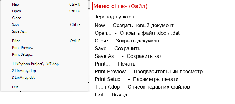
| Пункт | Горячая клавиша | Что делает |
|---|---|---|
| New (Создать) | Ctrl+N | Создаёт новый пустой документ-диаграмму |
| Open… (Открыть) | Ctrl+O | Открывает существующий .dop или .DAT файл |
| Close (Закрыть) | — | Закрывает текущее окно документа |
| Save (Сохранить) | Ctrl+S | Сохраняет текущий документ (.dop) вместе со всеми настройками оформления |
| Save As… (Сохранить как) | — | Сохраняет документ под новым именем |
| Print… (Печать) | Ctrl+P | Печатает диаграмму |
| Print Preview (Предпросмотр печати) | — | Показывает, как диаграмма будет выглядеть на бумаге |
| Print Setup… (Параметры печати) | — | Настройки принтера и страницы |
| Список последних файлов (MRU) | — | Быстрое открытие недавно использованных документов |
| Exit (Выход) | — | Закрывает программу |
При сохранении настройки оформления (цвета, шрифт, типы линий) дополнительно запоминаются в реестре Windows и используются как значения по умолчанию для новых документов.
5.2. Меню Edit (Правка)
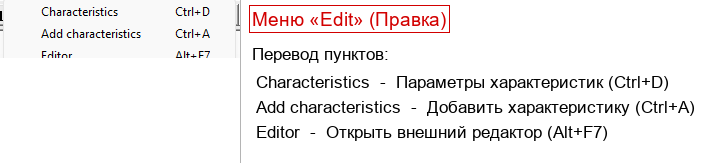
| Пункт | Горячая клавиша | Что делает |
|---|---|---|
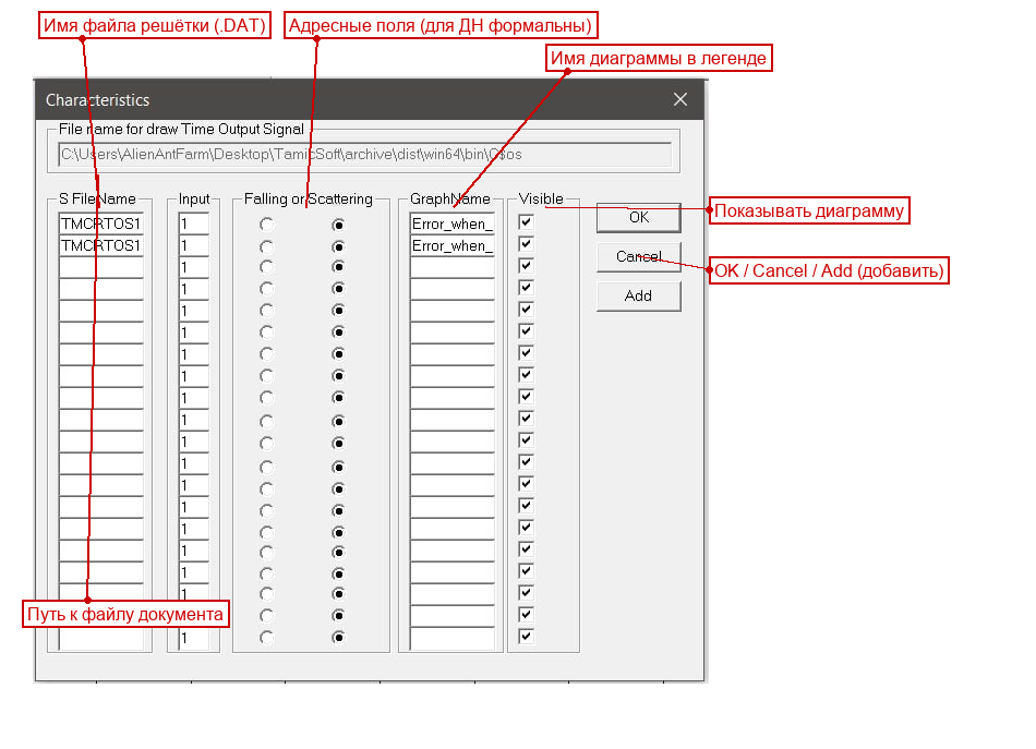
| Characteristics (Параметры документа / таблица диаграмм) | Ctrl+D | Открывает таблицу содержимого документа: список всех диаграмм. Для каждой видно имя графика, имя .DAT-файла, флаг «показывать/не показывать». Отсюда же открываются специфичные для ДН функции — девиации и сравнение с требуемой ДН (см. раздел 6) |
| Add characteristics (Добавить характеристику) | Ctrl+A | Открывает диалог выбора .DAT-файла и добавляет из него новую диаграмму в текущий документ |
| Editor (Внешний редактор) | Alt+F7 | Открывает файл документа во внешнем текстовом редакторе — для ручного редактирования .dop |
Важно: специфичные для диаграмм направленности диалоги (внесение девиаций, расчёт ДН отклонённой решётки относительно требуемой ДН) открываются не из верхнего меню, а из диалога Characteristics (Ctrl+D) — у него в TMC_DN добавлены отдельные кнопки. См. раздел 6.4–6.5.
Диалог Characteristics (таблица диаграмм документа):
5.3. Меню View (Вид)
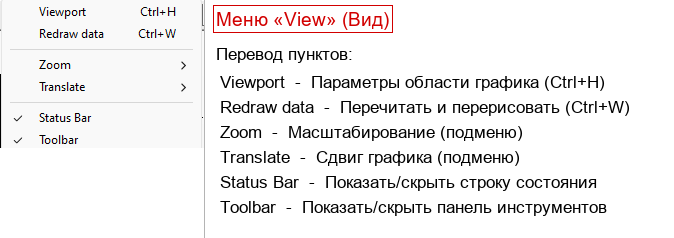
| Пункт | Горячая клавиша | Что делает |
|---|---|---|
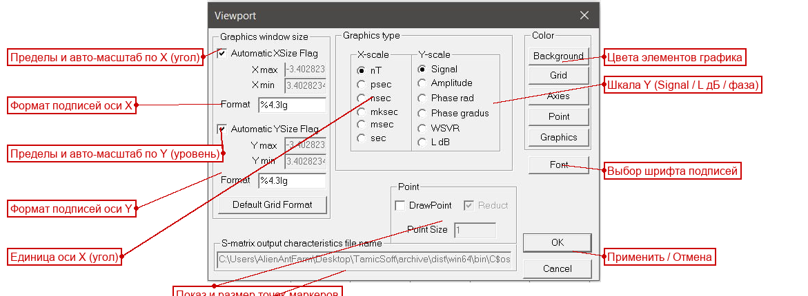
| Viewport (Параметры окна) | Ctrl+H | Открывает диалог настройки отображения: пределы Xmin/Xmax/Ymin/Ymax, авто-масштаб, формат подписей, показ точек-маркеров |
| Redraw data (Перечитать и перерисовать) | Ctrl+W | Заново читает данные и пересчитывает/перерисовывает диаграмму. Полезно, если изменилось описание решётки |
Диалог Viewport (параметры окна):
 | Zoom ► (Масштаб) | — | Подменю масштабирования (см. ниже) |
| Translate ► (Сдвиг) | — | Подменю сдвига границ области (см. ниже) |
| Status Bar (Строка состояния) | — | Включает/выключает нижнюю строку состояния |
| Toolbar (Панель инструментов) | — | Включает/выключает панель инструментов |
| Zoom ► (Масштаб) | — | Подменю масштабирования (см. ниже) |
| Translate ► (Сдвиг) | — | Подменю сдвига границ области (см. ниже) |
| Status Bar (Строка состояния) | — | Включает/выключает нижнюю строку состояния |
| Toolbar (Панель инструментов) | — | Включает/выключает панель инструментов |
Подменю View → Zoom (Масштаб)
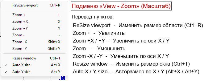
| Пункт | Горячая клавиша | Что делает |
|---|---|---|
| ReSize viewport (Подогнать область) | Ctrl+R | Подгоняет область рисования под текущее окно |
| Zoom + (Увеличить) | — | Увеличивает масштаб по обеим осям |
| Zoom +X (Увеличить по X) | — | Увеличивает масштаб только по углу |
| Zoom +Y (Увеличить по Y) | — | Увеличивает масштаб только по вертикали |
| Zoom − (Уменьшить) | — | Уменьшает масштаб по обеим осям |
| Zoom −X (Уменьшить по X) | Shift+X | Уменьшает масштаб по углу |
| Zoom −Y (Уменьшить по Y) | Shift+Y | Уменьшает масштаб по вертикали |
| Resize window (Подогнать окно данных) | Ctrl+T | Изменяет вещественные пределы окна данных |
| Auto X size (Авто-масштаб X) | Alt+X | Включает автоматический подбор пределов по X. В меню появляется галочка |
| Auto Y size (Авто-масштаб Y) | Alt+Y | Включает автоматический подбор пределов по Y. В меню появляется галочка |
При включённом авто-масштабе по оси программа сама подбирает пределы под минимум/максимум данных, и ручные пределы по этой оси игнорируются (поля Xmin/Xmax или Ymin/Ymax в диалоге Viewport становятся недоступны).
Подменю View → Translate (Сдвиг)

| Пункт | Что делает |
|---|---|
| Change Xmax, Xmin ► | Вложенное подменю: сдвинуть/изменить верхнюю и нижнюю границы по X (углу), а также перейти к началу/концу диапазона. Сдвиг выполняется шагами (порядка 10 % диапазона) |
| Change Ymax, Ymin ► | Вложенное подменю: сдвинуть/изменить верхнюю и нижнюю границы по Y (уровню). Сдвиг шагами (порядка 10 % диапазона) |
Сдвиг удобен, когда нужно «прокрутить» диаграмму влево/вправо/вверх/вниз, не меняя масштаб. Те же действия дают кнопки сдвига на панели инструментов (№16–21).
5.4. Меню Config (Настройки)
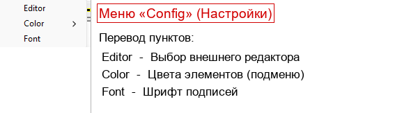
| Пункт | Что делает |
|---|---|
| Editor (Редактор) | Задаёт путь к внешнему текстовому редактору для .dop-файлов |
| Color ► (Цвет) | Подменю выбора цветов элементов графика (см. ниже) |
| Font (Шрифт) | Открывает стандартный диалог выбора шрифта, размера и цвета подписей осей и сетки |
Подменю Config → Color (Цвет)
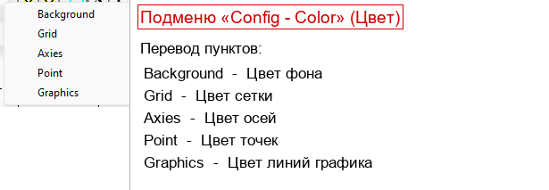
| Пункт | Что меняет |
|---|---|
| Background (Фон) | Цвет фона области графика |
| Grid (Сетка) | Цвет координатной сетки |
| Axies (Оси) | Цвет осей координат |
| Point (Точки) | Цвет точек-маркеров на кривых |
| Graphics (Графики) | Открывает диалог цветов/типов/толщины линий сразу для 16 кривых — здесь же можно задать индивидуальный цвет каждой диаграммы |
Пункт Graphics открывает таблицу из 16 образцов линий. Нажав на нужный образец, вы выбираете цвет, стиль (сплошная, пунктир, точки) и толщину этой линии.
5.5. Меню Window (Окно)
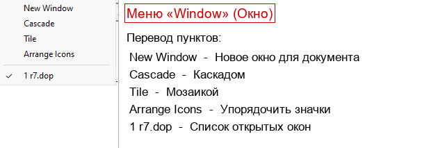
| Пункт | Что делает |
|---|---|
| New Window (Новое окно) | Открывает ещё одно окно для того же документа (полезно для разных масштабов одной диаграммы) |
| Cascade (Каскад) | Располагает окна каскадом |
| Tile (Мозаика) | Располагает окна плиткой (рядом) |
| Arrange Icons (Упорядочить значки) | Выравнивает свёрнутые окна-значки |
| Список окон | Переключение между открытыми окнами документов |
5.6. Меню Help (Справка)

| Пункт | Что делает |
|---|---|
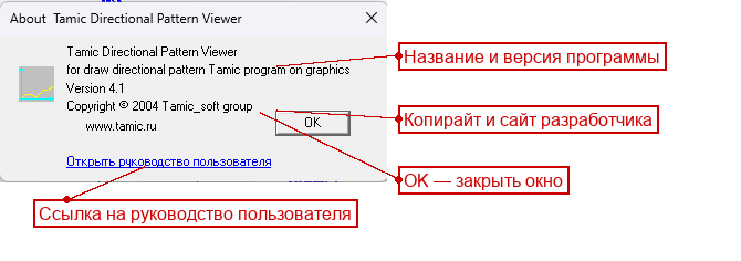
| About TMC_DN… (О программе) | Показывает окно с названием и версией программы (Tamic Directional Pattern Viewer) |
6. Типовые сценарии работы
Ниже — пошаговые инструкции для самых частых задач.
6.1. Открыть документ .dop
- Меню File → Open… (или Ctrl+O, или кнопка «Открыть» на панели).
- Выберите файл с расширением
.dop(например,r7.dop). - Программа рассчитает диаграмму направленности. Если решётка большая, появится окно прогресса с двумя индикаторами — дождитесь окончания расчёта.
- Диаграмма построится автоматически. Если кривая «уехала» за пределы окна — нажмите кнопки авто-масштаба Auto X size и Auto Y size.
6.2. Построить диаграмму по «сырому» описанию .DAT
- Меню File → Open… (Ctrl+O).
- В диалоге выберите файл с расширением
.DAT(например,r7.DAT). - Программа прочитает описание решётки, рассчитает диаграмму направленности (для большой решётки — с окном прогресса) и построит график; рядом будет создан документ для хранения настроек отображения. Сохраните его (File → Save, Ctrl+S), чтобы в следующий раз открывать уже готовый документ
.dop.
6.3. Прочитать КНД, КИП и излучённую мощность
После того как диаграмма рассчитана и построена:
- Посмотрите в правую панель строки состояния (внизу окна) — там выводятся КНД (
Knd, в том числе в дБ) и КИП (Kip). - Для крупной решётки вместо КИП показывается Emitted Power (излучённая мощность).
Что означают эти величины (для пользователя):
- КНД (коэффициент направленного действия, Knd) — насколько «остро» антенна излучает в главном направлении по сравнению с антенной, излучающей одинаково во все стороны. Чем больше КНД, тем у́же и сильнее главный лепесток. Часто выражается в децибелах (дБ): чем больше дБ, тем направленнее антенна.
- КИП (коэффициент использования поверхности, Kip) — мера того, насколько эффективно «работает» вся апертура (поверхность) антенны. Грубо: показывает, близка ли реальная решётка к идеальной по форме амплитудно-фазового распределения.
- Emitted Power (излучённая мощность) — суммарная мощность, излучаемая решёткой; программа выводит её вместо КИП для крупных решёток.
6.4. Внести случайные отклонения (девиации) в решётку
Эта функция позволяет смоделировать, как на диаграмму направленности влияют неточности изготовления антенны: небольшие отклонения координат, амплитуд и фаз отдельных излучателей.
- Откройте документ или
.DAT-файл с описанием решётки. - Откройте таблицу документа: меню Edit → Characteristics (Ctrl+D) или кнопка «Параметры документа» на панели.
- В этом диалоге найдите кнопку запуска функции девиаций и нажмите её. Откроется отдельный диалог внесения отклонений.
- В диалоге девиаций задаются:
- исходный файл решётки (
.DAT, источник); - выходной файл (.DAT, куда сохранить отклонённую решётку); - разброс координат излучателей по X и по Y (в миллиметрах); - разброс амплитуды (в процентах); - разброс фазы (в градусах). - Программа создаст новый файл решётки, в котором параметры каждого излучателя случайно отклонены в заданных пределах (равномерное распределение). Этот новый
.DATможно открыть в TMC_DN и сравнить его диаграмму с исходной.
6.5. Сравнить ДН отклонённой решётки с требуемой (эталонной)
Эта функция считает диаграмму направленности для заданного амплитудно-фазового распределения и сохраняет её рядом с требуемой (эталонной) ДН в одном файле сравнения, чтобы их было удобно сопоставить.
- Откройте таблицу документа: Edit → Characteristics (Ctrl+D).
- В диалоге найдите кнопку запуска функции сравнения с требуемой ДН и нажмите её. Откроется отдельный диалог расчёта.
- В диалоге задаются:
- файл распределения амплитуд/фаз решётки (
.DAT); - файл требуемой (эталонной) ДН — задаёт, какую диаграмму вы хотите получить в идеале; - выходной файл сравнения, в который запишутся две диаграммы (требуемая и фактически рассчитанная) для каждого угла. - Программа рассчитает диаграмму для заданного распределения и запишет файл сравнения. Его можно открыть и увидеть, насколько фактическая ДН отличается от требуемой.
6.6. Настроить масштаб (Zoom / Auto X / Auto Y)
Есть три способа изменить масштаб:
- Мышью — зажмите левую кнопку и обведите прямоугольником интересующую область диаграммы; при отпускании кнопки программа увеличит выделенное. Двойной щелчок в области графика подгоняет масштаб обратно.
- Кнопками панели — Zoom + / Zoom − (обе оси), Zoom +X/−X, Zoom +Y/−Y (по одной оси).
- Авто-масштаб — View → Zoom → Auto X size (Alt+X) и Auto Y size (Alt+Y). Программа сама подберёт пределы так, чтобы видеть всю диаграмму. Это самый быстрый способ «вписать» график в окно.
6.7. Сдвинуть диаграмму (Translate)
- Меню View → Translate.
- Выберите Change Xmax, Xmin (сдвиг по углу) или Change Ymax, Ymin (сдвиг по уровню).
- Во вложенном подменю выберите увеличение или уменьшение нужной границы. Диаграмма сдвинется шагом порядка 10 % диапазона.
Тот же эффект дают кнопки сдвига на панели инструментов (№16–21).
Сдвиг работает только при выключенном авто-масштабе по соответствующей оси: при включённом авто-масштабе пределы определяются автоматически по данным.
6.8. Сменить цвета и оформление
Цвет фона / сетки / осей / точек: 1. Меню Config → Color → Background / Grid / Axies / Point. 2. В стандартном диалоге выберите цвет → OK.
Цвет, стиль и толщина кривых: 1. Меню Config → Color → Graphics. 2. В открывшейся таблице нажмите образец нужной диаграммы. 3. Выберите цвет, стиль линии (сплошная/пунктир/точки) и толщину → OK.
Шрифт подписей: 1. Меню Config → Font. 2. Выберите шрифт, размер и цвет → OK.
6.9. Напечатать диаграмму
- Сначала настройте масштаб и оформление так, как хотите видеть на бумаге.
- (По желанию) Меню File → Print Preview — проверьте, как диаграмма ляжет на страницу.
- Меню File → Print… (Ctrl+P) или кнопка «Печать».
- Выберите принтер и нажмите OK.
7. Форматы входных данных
TMC_DN работает с документом .dop, файлом описания решётки .DAT, а также с файлами распределения .AMP (амплитуды) и .FAZ (фазы).
7.1. Файл документа .dop
.dop — это текстовый файл-документ TMC_DN. Его можно открыть любым текстовым редактором. Он хранит настройки оформления и список диаграмм, но не хранит сами данные — данные берутся из файлов .DAT, на которые ссылается документ.
Структура файла (на примере реального файла samples/SAMPLE_R/KIRILL/HIPERSOUND/r7.dop):
#TMCGROTS
!Graphics parameters
!Graphics data
!file name : E:\BackUP\ARHIV\WORK\Source\SAMPLE_R\KIRILL\HIPERSOUND\r7.dop
!Data file for draw graphics
!TFileName GraphicsName DrawFlag Input1 Mod1 Input2 Mod2
r7.DAT r7.DAT 1 1 1 1 1
Разбор по строкам:
| Строка | Назначение |
|---|---|
#TMCGROTS |
Сигнатура — обязательная первая строка. По ней программа узнаёт «свой» файл документа (она такая же, как у документов TMCROS, поскольку TMC_DN построен на той же кодовой базе) |
Строки, начинающиеся с ! |
Комментарии — программа их игнорирует (включая авто-сгенерированный путь и подсказку по столбцам) |
Строки #Ключ значение |
Параметры оформления (в этом простом примере их нет, но они могут присутствовать — пределы осей, цвета, шрифт; по аналогии с документами TMCGROUT/TMCROS) |
Последние строки (без #) |
Описания диаграмм — по одной строке на диаграмму |
Описание диаграммы (строка данных). Формат столбцов указан в комментарии выше неё:
!TFileName GraphicsName DrawFlag Input1 Mod1 Input2 Mod2
r7.DAT     r7.DAT       1        1      1    1      1
| Столбец | Значение в примере | Назначение |
|---|---|---|
TFileName |
r7.DAT |
Имя файла описания решётки (обычно относительный путь рядом с .dop) |
GraphicsName |
r7.DAT |
Подпись диаграммы в легенде |
DrawFlag |
1 |
Показывать диаграмму: 1 — да, 0 — нет |
Input1, Mod1, Input2, Mod2 |
1 1 1 1 |
Адресные поля, унаследованные от общего формата вьюверов. Для ДН значимым является основной адрес; остальные при чтении приводятся к значениям по умолчанию |
7.2. Файл описания антенной решётки .DAT
.DAT — это файл с описанием антенной решётки, по которому программа рассчитывает диаграмму направленности. По описанию в API-документации (docs/api/viewers/tmc_dn.md, метод c2DArray::ReadData) это текстовый файл со следующей структурой:
Frequence = <частота> Ghz;
N = <число излучателей>;
<выражение собственной ДН одного элемента>
0   X = <x0> mm; Y = <y0> mm; Amplitude = <a0>; Faza = <f0> degree; [FiMin = ... degree; FiMax = ... degree; <выражение>]
1   X = <x1> mm; Y = <y1> mm; Amplitude = <a1>; Faza = <f1> degree; ...
...
Разбор по строкам:
| Строка | Назначение | Единицы |
|---|---|---|
Frequence = … Ghz; |
Рабочая частота антенны | ГГц (внутри программы переводится в Гц) |
N = …; |
Число излучателей в решётке | целое |
| 3-я строка — выражение | Собственная диаграмма направленности одного элемента (формула). Вычисляется библиотекой exprint. Изотропный (всенаправленный) элемент задаётся как 1.; направленный — выражениями вида sin(f), cos(f) и т.п., где f — угол |
угол в радианах |
| Строки излучателей (по одной на элемент) | Для каждого излучателя: его номер, координаты X/Y, амплитуда Amplitude, фаза Faza. Необязательно — угловой диапазон видимости элемента FiMin/FiMax и собственное выражение ДН |
X, Y — мм (внутри → метры); Faza, FiMin, FiMax — градусы (внутри → радианы) |
Что за что отвечает:
- Координаты
X,Yизлучателя задают его положение в плоскости решётки. Именно от взаимного расположения элементов зависит, как складываются их поля по разным углам и какой получается главный лепесток. Amplitude— амплитуда возбуждения элемента (насколько «громко» излучает данный элемент). Распределение амплитуд по решётке влияет на уровень боковых лепестков.Faza— фаза возбуждения элемента (в градусах). Фазовое распределение позволяет «наклонять» главный лепесток (сканирование лучом).- Выражение собственной ДН элемента (3-я строка и/или в строке элемента) задаёт, как излучает один отдельный элемент в зависимости от угла. Это формула на языке библиотеки
exprint(доступны тригонометрические и другие функции; угол обозначается переменной угла). FiMin/FiMax(если заданы) ограничивают угловой диапазон, в котором элемент считается «видимым» (излучающим).
7.3. Файлы распределения .AMP и .FAZ
.AMP и .FAZ — это амплитудное и фазовое распределения по элементам (раскрыву) антенны: «карта» того, с какой амплитудой и фазой возбуждается каждая точка апертуры. Из них формируется возбуждение излучателей решётки.
Из доступных файлов видно следующее (на примере r7.AMP):
| Ключ заголовка | Значение в примере | Предполагаемый смысл |
|---|---|---|
#TMC_GraphicsOutputFieldFile FormVer2.0 2000 |
— | Сигнатура файла распределения поля (версия формата 2.0) |
#TMCGROFLD_nT 1930 |
1930 | Номер временно́го шага, на котором сохранено распределение |
#TMCGROFLD_Time 9.10441e-009 |
9.1 нс | Момент времени |
#TMCGROFLD_Delta 0.002 |
0.002 | Шаг сетки |
#TMCGROFLD_Xmin 0, #TMCGROFLD_Ymin 0 |
0 | Начало координат области |
#TMCGROFLD_Accuracy 8 |
8 | Размер числа в байтах: 8 — double (двойная точность, текущая сборка), 4 — float |
#TMCGROFLD_LongUnit mm 0.001 |
мм | Единица длины (миллиметры) |
#TMCGROFLD_TimeUnit ns 1e-009 |
нс | Единица времени (наносекунды) |
#TMCGROFLD_nX 502, #TMCGROFLD_nY 502 |
502 × 502 | Размер сетки распределения |
| Далее | бинарные данные | Двумерный массив значений поля (амплитуды — в .AMP, фазы — в .FAZ) |
Файлы
.AMP/.FAZв таком виде не предназначены для ручного редактирования — после заголовка идут бинарно записанные числа. Открывать их следует средствами пакета, а не текстовым редактором.
7.4. Как получить файлы данных для TMC_DN
Данные для диаграммы направленности готовит счётное ядро при расчёте планарной структуры. Кратко (подробно — в docs/api/kernels/planar_rt_h.md и docs/api/libs/tmcindan.md):
- Подготовьте входной файл-шаблон
.tpl(топология структуры, параметры, секция вывода) и рассчитайте структуру в ядреtmc_rth.exe(H-поляризация). В процессе расчёта ядро интегрирует поле по времени (классCFieldIntegrated). - Ядро выполняет экспорт данных для диаграммы направленности функцией
CFieldIntegrated::ExportToDirectionalPattern(TMCIndan): по накопленному полю вычисляются амплитуда и фаза излучателей вдоль границ области (Xmin/Xmax/Ymin/Ymax). На этом этапе и формируются файлы амплитудного/фазового распределения и описание решётки. - Полученные файлы открываются в TMC_DN, где по ним строится и анализируется диаграмма направленности.
Готовые примеры для тренировки лежат в samples/SAMPLE_R/KIRILL/HIPERSOUND/ (r7.dop, r7.DAT, r7.AMP, r7.FAZ).
8. Возможные проблемы и их решение
| Симптом | Причина | Что делать |
|---|---|---|
| Долгий расчёт, окно прогресса висит | Большая решётка считается в фоновом потоке | Дождитесь окончания: следите за двумя индикаторами (готовность текущей ДН и по всем ДН). Расчёт большой решётки объективно длительный |
| В легенде/области графика надпись об ошибке чтения | Файл .DAT не найден, пуст или повреждён |
Проверьте, существует ли .DAT-файл по указанному в .dop пути; подготовьте его заново |
| Сообщение об ошибке выражения ДН элемента | Неверная формула в 3-й строке .DAT (выражение exprint) |
Проверьте синтаксис выражения собственной ДН элемента; для всенаправленного элемента используйте 1. |
| Диаграмма пустая или кривая не видна | Включён неудачный масштаб, либо данные вне окна | Нажмите Auto X size и Auto Y size (Alt+X, Alt+Y), чтобы вписать диаграмму в окно |
| Диаграмма есть, но «уезжает» за край | Заданы ручные пределы Xmin/Xmax/Ymin/Ymax | Откройте View → Viewport и проверьте пределы, либо включите авто-масштаб |
| После изменения описания решётки диаграмма не обновилась | TMC_DN показывает старые данные | Нажмите View → Redraw data (Ctrl+W) или кнопку «Перерисовать» — диаграмма пересчитается |
| Кривая одного цвета с фоном/её плохо видно | Совпали цвета | Config → Color → Graphics — задайте контрастный цвет линии |
| Не открывается файл — сообщение про «не тот формат» | Первая строка документа не #TMCGROTS |
Убедитесь, что открываете корректный документ .dop (первая строка должна быть #TMCGROTS) либо корректный .DAT |
User manual — the TMC_DN program (TMC_DN.exe)
TMC Suite package. This manual is written in plain language and is intended for a user seeing the program for the first time. All menu and button names are given as they appear in the program (the interface is in English), with a translation and explanation next to them.
1. Purpose of the program
TMC_DN (the executable TMC_DN.exe, full name Tamic Directional Pattern
Viewer) is a program for computing and viewing the radiation patterns (RP) of
antennas and antenna arrays. In simple terms, it builds a graph where:
- the horizontal axis (X) shows the angle (in radians, roughly from −π to +π) — that is, the direction in space the antenna "looks" at;
- the vertical axis (Y) shows the radiation-pattern level (Pattern) — how strongly the antenna radiates (or receives) in that direction.
A radiation pattern is a "map" of how the antenna distributes radiation over angles: in which directions it radiates strongly (the main lobe) and in which weakly (the side lobes and nulls). For an antenna array (a set of radiators placed in space), the shape of the pattern depends on the coordinates of the elements, their amplitudes and phases. TMC_DN takes the description of such an array, computes its radiation pattern and draws it as a clear graph.
What the program can do:
- open ready-made pattern documents (
.dopfiles) or array-description files (.DAT) directly; - compute the radiation pattern of an antenna array from a description of its radiators (coherent summation of the fields of all elements over the angle);
- compute and show the integral characteristics of the antenna: the directivity (Knd, including in decibels), the aperture efficiency (Kip), and for large arrays the emitted power (Emitted Power);
- show several patterns at once on one field (for example, patterns of different arrays for comparison);
- change the scale (zoom in/out, auto-fit by axes), shift the visible area;
- configure the colors of the background, grid, axes and the curves themselves, as well as the label font;
- introduce random deviations into the radiator parameters — coordinates, amplitudes, phases — and see how the pattern "degrades"; compare the resulting pattern with the required (reference) pattern;
- print the pattern and save the display settings in the
.dopdocument itself.
Computing a large array can take a noticeable amount of time, so TMC_DN computes the pattern in the background and shows a progress window with two indicators (the readiness of the current pattern and the readiness across all patterns of the document). Details in section 6.
How does TMC_DN differ from the "neighboring" programs of the package? TMCGROUT shows frequency characteristics (the S-matrix as a function of frequency), TMCROS shows time signals, and TMC_DN shows radiation patterns (the radiation level as a function of angle). Outwardly all three are very similar (built to the same design), so their menus and toolbars are almost identical. But TMC_DN can additionally compute the array pattern, compute directivity/aperture efficiency, and model deviations — the other viewers cannot.
2. Launching and opening data
How to launch the program
- Find the file
TMC_DN.exe(after the build it is indist/win32/binordist/win64/bin). - Launch it with a double click.
- On the first launch the program maximizes to full screen. If any files were
opened before, TMC_DN will try to automatically open the last of them (the
"recent files" list is stored in the Windows registry under
TMC_DN).
Which file to open
TMC_DN works with two main file types (details in section 7):
| File | What it is | When to open |
|---|---|---|
.dop |
TMC_DN document: a text file with pattern settings and a reference to the array-description file(s) | The usual way. Saves colors, scale, list of patterns |
.DAT |
Antenna-array description file (frequency, radiators, element-pattern expression) | If you want to build a pattern from a "raw" description. The program will create a document for it itself |
To open a file:
- Menu File → Open…, or click the "Open" button on the toolbar, or press Ctrl+O.
- In the dialog select the desired
.dopor.DATfile. - The program computes the radiation pattern (for a large array a progress window appears) and builds the graph.
If you open a
.DATfile, a document will be created next to it (it stores the display settings). In the future it is more convenient to open the.dopdocument.
3. The main window
The main window is a multiple-document window (MDI): several windows with different patterns can be open inside it at once.
The window consists of four zones:
- Menu bar (top) — all program commands, grouped into sections (File, Edit, View, Config, Window, Help). Details in section 5.
- Toolbar — a row of icon buttons for the most frequent actions. Details in section 4.
- Graph area (center) — here the axes, the coordinate grid and the radiation pattern itself are drawn. The horizontal axis shows the angle (radians), the vertical the pattern level. The mouse works over this area: you can select a rectangle to zoom in, and a double click fits the scale.
- Status bar (bottom) — two panels:
- the left one — the coordinates of the point under the mouse cursor (the
angle value on X and the pattern-level value on Y);
- the right one — the integral characteristics of the current pattern: the
directivity (
Knd, including in dB) and the aperture efficiency (Kip), and for a large array the emitted power (Emitted Power) instead of Kip.
4. The toolbar
The toolbar duplicates the most frequent menu commands as buttons. If the toolbar
is not visible, enable it via View → Toolbar. TMC_DN's toolbar and menu are
shared with TMCGROUT — the radiation-pattern program (the DiaNapGr module)
has no resource file of its own, so the set of buttons is the same.
The buttons go from left to right. Below is the purpose of each.
| # | Button | Name (Eng.) | Shortcut | What it does |
|---|---|---|---|---|
| 1 | |
Open | Ctrl+O | Opens a .dop or .DAT file (same as File → Open) |
| 2 | |
Add characteristics | Ctrl+A | Adds one more pattern from a selected .DAT file to the document |
| 3 | |
Characteristics | Ctrl+D | Opens the table-list of all patterns in the document (names, files, display flags); the deviation functions are also available here — see section 6 |
| 4 | |
Viewport | Ctrl+H | Opens the display-settings dialog: axis limits, auto-scale, label format, points |
| 5 | |
Redraw data | Ctrl+W | Re-reads the data and recomputes/redraws the pattern |
| 6 | |
Resize viewport | Ctrl+R | Fits the drawing area to the window size |
| 7 | |
Zoom + | — | Zooms in on both axes |
| 8 | |
Zoom +X | — | Zooms in only horizontally (angle) |
| 9 | |
Zoom +Y | — | Zooms in only vertically (level) |
| 10 | |
Zoom − | — | Zooms out on both axes |
| 11 | |
Zoom −X | Shift+X | Zooms out horizontally |
| 12 | |
Zoom −Y | Shift+Y | Zooms out vertically |
| 13 | |
Resize window | Ctrl+T | Fits the real limits (the data window) |
| 14 | |
Auto X size | Alt+X | Automatically fits the X-axis (angle) limits to the data |
| 15 | |
Auto Y size | Alt+Y | Automatically fits the Y-axis limits to the data |
| 16 | |
To start | — | Jump to the start of the X (angle) range |
| 17 | |
To end | — | Jump to the end of the X (angle) range |
| 18 | |
Shift X left | — | Shifts the visible area left along the angle |
| 19 | |
Shift X right | — | Shifts the visible area right along the angle |
| 20 | |
Shift Y down | — | Shifts the visible area down |
| 21 | |
Shift Y up | — | Shifts the visible area up |
| 22 | |
Ctrl+P | Prints the current pattern (same as File → Print) | |
| 23 | |
About | — | Shows the "About TMC_DN" window |
5. The menus
Below, every item of every menu is explained: what it does, its keyboard shortcut, and what happens after you select it. TMC_DN's menu is shared with TMCGROUT.
5.1. The File menu
| Item | Shortcut | What it does |
|---|---|---|
| New | Ctrl+N | Creates a new empty pattern document |
| Open… | Ctrl+O | Opens an existing .dop or .DAT file |
| Close | — | Closes the current document window |
| Save | Ctrl+S | Saves the current document (.dop) together with all display settings |
| Save As… | — | Saves the document under a new name |
| Print… | Ctrl+P | Prints the pattern |
| Print Preview | — | Shows how the pattern will look on paper |
| Print Setup… | — | Printer and page settings |
| Recent files list (MRU) | — | Quick opening of recently used documents |
| Exit | — | Closes the program |
When saving, the display settings (colors, font, line types) are additionally remembered in the Windows registry and used as defaults for new documents.
5.2. The Edit menu
| Item | Shortcut | What it does |
|---|---|---|
| Characteristics (document parameters / pattern table) | Ctrl+D | Opens the table of the document's contents: a list of all patterns. For each you can see the graph name, the .DAT-file name, the "show/hide" flag. The RP-specific functions — deviations and comparison with the required pattern — are also opened from here (see section 6) |
| Add characteristics | Ctrl+A | Opens a .DAT-file selection dialog and adds a new pattern from it to the current document |
| Editor (external editor) | Alt+F7 | Opens the document file in an external text editor — for manual editing of the .dop |
Important: the radiation-pattern-specific dialogs (introducing deviations, computing the pattern of a deviated array relative to the required pattern) are opened not from the top menu but from the Characteristics dialog (Ctrl+D) — separate buttons have been added to it in TMC_DN. See sections 6.4–6.5.
The Characteristics dialog (the document's pattern table):
5.3. The View menu
| Item | Shortcut | What it does |
|---|---|---|
| Viewport | Ctrl+H | Opens the display-settings dialog: limits Xmin/Xmax/Ymin/Ymax, auto-scale, label format, showing point markers |
| Redraw data | Ctrl+W | Re-reads the data and recomputes/redraws the pattern. Useful if the array description changed |
The Viewport dialog (window parameters):
| Item | Shortcut | What it does |
|---|---|---|
| Zoom ► | — | Zoom submenu (see below) |
| Translate ► | — | Submenu for shifting the area limits (see below) |
| Status Bar | — | Toggles the bottom status bar |
| Toolbar | — | Toggles the toolbar |
The View → Zoom submenu
| Item | Shortcut | What it does |
|---|---|---|
| ReSize viewport | Ctrl+R | Fits the drawing area to the current window |
| Zoom + | — | Zooms in on both axes |
| Zoom +X | — | Zooms in only on the angle |
| Zoom +Y | — | Zooms in only vertically |
| Zoom − | — | Zooms out on both axes |
| Zoom −X | Shift+X | Zooms out on the angle |
| Zoom −Y | Shift+Y | Zooms out vertically |
| Resize window | Ctrl+T | Changes the real limits of the data window |
| Auto X size | Alt+X | Enables automatic fitting of the X limits. A check mark appears in the menu |
| Auto Y size | Alt+Y | Enables automatic fitting of the Y limits. A check mark appears in the menu |
With auto-scale enabled on an axis, the program fits the limits to the minimum/maximum of the data itself, and manual limits on that axis are ignored (the Xmin/Xmax or Ymin/Ymax fields in the Viewport dialog become unavailable).
The View → Translate submenu
| Item | What it does |
|---|---|
| Change Xmax, Xmin ► | Nested submenu: shift/change the upper and lower X (angle) limits, and jump to the start/end of the range. The shift is performed in steps (about 10% of the range) |
| Change Ymax, Ymin ► | Nested submenu: shift/change the upper and lower Y (level) limits. Shift in steps (about 10% of the range) |
Shifting is convenient when you need to "scroll" the pattern left/right/up/down without changing the scale. The same actions are produced by the shift buttons on the toolbar (#16–21).
5.4. The Config menu
| Item | What it does |
|---|---|
| Editor | Sets the path to the external text editor for .dop files |
| Color ► | Submenu for choosing the colors of the graph elements (see below) |
| Font | Opens the standard dialog for choosing the font, size and color of the axis and grid labels |
The Config → Color submenu
| Item | What it changes |
|---|---|
| Background | The background color of the graph area |
| Grid | The color of the coordinate grid |
| Axies | The color of the coordinate axes |
| Point | The color of the point markers on the curves |
| Graphics | Opens a dialog with colors/types/thicknesses of lines for 16 curves at once — here you can also set an individual color for each pattern |
The Graphics item opens a table of 16 line samples. By clicking the desired sample, you choose the color, the style (solid, dashed, dotted) and the thickness of that line.
5.5. The Window menu
| Item | What it does |
|---|---|
| New Window | Opens another window for the same document (useful for different scales of one pattern) |
| Cascade | Arranges the windows in a cascade |
| Tile | Arranges the windows tiled (side by side) |
| Arrange Icons | Aligns the minimized window icons |
| Windows list | Switches between the open document windows |
5.6. The Help menu
| Item | What it does |
|---|---|
| About TMC_DN… | Shows a window with the program name and version (Tamic Directional Pattern Viewer) |
6. Typical workflows
Below are step-by-step instructions for the most frequent tasks.
6.1. Open a .dop document
- Menu File → Open… (or Ctrl+O, or the "Open" button on the toolbar).
- Select a file with the
.dopextension (for example,r7.dop). - The program computes the radiation pattern. If the array is large, a progress window with two indicators appears — wait for the computation to finish.
- The pattern is built automatically. If the curve has "run off" beyond the window, press the auto-scale buttons Auto X size and Auto Y size.
6.2. Build a pattern from a "raw" description .DAT
- Menu File → Open… (Ctrl+O).
- In the dialog select a file with the
.DATextension (for example,r7.DAT). - The program reads the array description, computes the radiation pattern (for a
large array — with a progress window) and builds the graph; a document to store
the display settings is created next to it. Save it (File → Save, Ctrl+S) so
that next time you open the ready
.dopdocument.
6.3. Read the directivity, aperture efficiency and emitted power
After the pattern is computed and built:
- Look at the right panel of the status bar (bottom of the window) — the
directivity (
Knd, including in dB) and the aperture efficiency (Kip) are shown there. - For a large array, Emitted Power is shown instead of Kip.
What these quantities mean (for the user):
- Directivity (Knd) — how "sharply" the antenna radiates in the main direction compared with an antenna radiating equally in all directions. The higher the directivity, the narrower and stronger the main lobe. It is often expressed in decibels (dB): the more dB, the more directional the antenna.
- Aperture efficiency (Kip) — a measure of how efficiently the whole aperture (surface) of the antenna "works". Roughly: it shows how close the real array is to the ideal in the shape of the amplitude-phase distribution.
- Emitted Power — the total power radiated by the array; the program shows it instead of Kip for large arrays.
6.4. Introduce random deviations into the array
This function lets you model how manufacturing inaccuracies of an antenna affect the radiation pattern: small deviations of the coordinates, amplitudes and phases of individual radiators.
- Open a document or a
.DATfile with the array description. - Open the document table: menu Edit → Characteristics (Ctrl+D) or the "Document parameters" button on the toolbar.
- In this dialog find the button that launches the deviations function and press it. A separate deviation dialog opens.
- In the deviation dialog you set:
- the source file of the array (
.DAT, the source); - the output file (.DAT, where to save the deviated array); - the coordinate spread of the radiators along X and Y (in millimeters); - the amplitude spread (as a percentage); - the phase spread (in degrees). - The program creates a new array file in which the parameters of each radiator
are randomly deviated within the given limits (a uniform distribution). This new
.DATcan be opened in TMC_DN and its pattern compared with the original.
Input: the source array file + the spread values (X, Y, amplitude, phase). Output: a new
.DATfile with randomly deviated radiator parameters.
6.5. Compare the pattern of a deviated array with the required (reference) one
This function computes the radiation pattern for a given amplitude-phase distribution and saves it next to the required (reference) pattern in a single comparison file, so that they are convenient to compare.
- Open the document table: Edit → Characteristics (Ctrl+D).
- In the dialog find the button that launches the comparison with the required pattern function and press it. A separate computation dialog opens.
- In the dialog you set:
- the array amplitude/phase distribution file (
.DAT); - the required (reference) pattern file — it defines which pattern you want to obtain ideally; - the output comparison file, into which two patterns (the required and the actually computed) are written for each angle. - The program computes the pattern for the given distribution and writes the comparison file. It can be opened to see how much the actual pattern differs from the required one.
Input: the amplitude/phase distribution file + the required-pattern file. Output: a comparison file with three columns — angle · required pattern · computed pattern.
6.6. Adjust the scale (Zoom / Auto X / Auto Y)
There are three ways to change the scale:
- With the mouse — hold the left button and draw a rectangle around the pattern area of interest; when you release the button the program zooms in on the selection. A double click in the graph area fits the scale back.
- With the toolbar buttons — Zoom + / Zoom − (both axes), Zoom +X/−X, Zoom +Y/−Y (one axis).
- Auto-scale — View → Zoom → Auto X size (Alt+X) and Auto Y size (Alt+Y). The program fits the limits so that the whole pattern is visible. This is the fastest way to "fit" the graph into the window.
6.7. Shift the pattern (Translate)
- Menu View → Translate.
- Select Change Xmax, Xmin (shift along the angle) or Change Ymax, Ymin (shift along the level).
- In the nested submenu, choose to increase or decrease the desired limit. The pattern shifts by a step of about 10% of the range.
The same effect is produced by the shift buttons on the toolbar (#16–21).
The shift only works with auto-scale disabled on the corresponding axis: with auto-scale enabled, the limits are determined automatically from the data.
6.8. Change the colors and appearance
Background / grid / axes / point color: 1. Menu Config → Color → Background / Grid / Axies / Point. 2. In the standard dialog select the color → OK.
Curve color, style and thickness: 1. Menu Config → Color → Graphics. 2. In the opened table click the sample of the desired pattern. 3. Select the color, the line style (solid/dashed/dotted) and the thickness → OK.
Label font: 1. Menu Config → Font. 2. Select the font, size and color → OK.
6.9. Print the pattern
- First set the scale and appearance the way you want to see them on paper.
- (Optional) Menu File → Print Preview — check how the pattern will fit on the page.
- Menu File → Print… (Ctrl+P) or the "Print" button.
- Select the printer and click OK.
7. Input data formats
TMC_DN works with the .dop document, the .DAT array-description file, and the
distribution files .AMP (amplitudes) and .FAZ (phases).
7.1. The .dop document file
.dop is a text TMC_DN document file. It can be opened with any text editor.
It stores the display settings and the list of patterns, but does not store the
data itself — the data is taken from the .DAT files referenced by the document.
File structure (using the real file
samples/SAMPLE_R/KIRILL/HIPERSOUND/r7.dop):
#TMCGROTS
!Graphics parameters
!Graphics data
!file name : E:\BackUP\ARHIV\WORK\Source\SAMPLE_R\KIRILL\HIPERSOUND\r7.dop
!Data file for draw graphics
!TFileName GraphicsName DrawFlag Input1 Mod1 Input2 Mod2
r7.DAT r7.DAT 1 1 1 1 1
Line-by-line breakdown:
| Line | Purpose |
|---|---|
#TMCGROTS |
Signature — the mandatory first line. The program recognizes "its" document file by it (it is the same as for TMCROS documents, since TMC_DN is built on the same codebase) |
Lines starting with ! |
Comments — the program ignores them (including the auto-generated path and the column hint) |
#Key value lines |
Display parameters (there are none in this simple example, but they may be present — axis limits, colors, font; by analogy with TMCGROUT/TMCROS documents) |
The last lines (without #) |
Pattern descriptions — one line per pattern |
Pattern description (a data line). The column format is given in the comment above it:
!TFileName GraphicsName DrawFlag Input1 Mod1 Input2 Mod2
r7.DAT     r7.DAT       1        1      1    1      1
| Column | Value in the example | Purpose |
|---|---|---|
TFileName |
r7.DAT |
The array-description file name (usually a relative path next to the .dop) |
GraphicsName |
r7.DAT |
The pattern caption in the legend |
DrawFlag |
1 |
Show the pattern: 1 — yes, 0 — no |
Input1, Mod1, Input2, Mod2 |
1 1 1 1 |
Address fields inherited from the common viewer format. For the pattern the main address is significant; the rest are reduced to default values when reading |
7.2. The .DAT antenna-array description file
.DAT is a file with the description of the antenna array from which the
program computes the radiation pattern. According to the description in the API
documentation (docs/api/viewers/tmc_dn.md, the c2DArray::ReadData method), it
is a text file with the following structure:
Frequence = <frequency> Ghz;
N = <number of radiators>;
<expression of the element's own pattern>
0   X = <x0> mm; Y = <y0> mm; Amplitude = <a0>; Faza = <f0> degree; [FiMin = ... degree; FiMax = ... degree; <expression>]
1   X = <x1> mm; Y = <y1> mm; Amplitude = <a1>; Faza = <f1> degree; ...
...
Line-by-line breakdown:
| Line | Purpose | Units |
|---|---|---|
Frequence = … Ghz; |
The operating frequency of the antenna | GHz (converted to Hz inside the program) |
N = …; |
The number of radiators in the array | integer |
| 3rd line — an expression | The radiation pattern of a single element (a formula). Evaluated by the exprint library. An isotropic (omnidirectional) element is given as 1.; a directional one by expressions of the form sin(f), cos(f), etc., where f is the angle |
angle in radians |
| Radiator lines (one per element) | For each radiator: its number, coordinates X/Y, amplitude Amplitude, phase Faza. Optionally — the angular visibility range of the element FiMin/FiMax and its own pattern expression |
X, Y — mm (internally → meters); Faza, FiMin, FiMax — degrees (internally → radians) |
What is responsible for what:
- The coordinates
X,Yof a radiator set its position in the plane of the array. It is precisely the mutual arrangement of the elements that determines how their fields add up at different angles and what main lobe results. Amplitude— the excitation amplitude of the element (how "loudly" the given element radiates). The distribution of amplitudes over the array affects the side-lobe level.Faza— the excitation phase of the element (in degrees). The phase distribution allows the main lobe to be "tilted" (beam scanning).- The element's own pattern expression (the 3rd line and/or in the element
line) sets how a single element radiates as a function of angle. It is a formula
in the
exprintlibrary language (trigonometric and other functions are available; the angle is denoted by the angle variable). FiMin/FiMax(if set) limit the angular range in which the element is considered "visible" (radiating).
7.3. The .AMP and .FAZ distribution files
.AMP and .FAZ are the amplitude and phase distributions over the
elements (aperture) of the antenna: a "map" of the amplitude and phase with which
each point of the aperture is excited. The excitation of the array radiators is
formed from them.
From the available files the following can be seen (using r7.AMP as an example):
| Header key | Value in the example | Presumed meaning |
|---|---|---|
#TMC_GraphicsOutputFieldFile FormVer2.0 2000 |
— | The signature of the field-distribution file (format version 2.0) |
#TMCGROFLD_nT 1930 |
1930 | The time-step number at which the distribution was saved |
#TMCGROFLD_Time 9.10441e-009 |
9.1 ns | The time moment |
#TMCGROFLD_Delta 0.002 |
0.002 | The grid step |
#TMCGROFLD_Xmin 0, #TMCGROFLD_Ymin 0 |
0 | The origin of the area |
#TMCGROFLD_Accuracy 8 |
8 | The number size in bytes: 8 — double (double precision, the current build), 4 — float |
#TMCGROFLD_LongUnit mm 0.001 |
mm | The length unit (millimeters) |
#TMCGROFLD_TimeUnit ns 1e-009 |
ns | The time unit (nanoseconds) |
#TMCGROFLD_nX 502, #TMCGROFLD_nY 502 |
502 × 502 | The size of the distribution grid |
| Then | binary data | A two-dimensional array of field values (amplitudes in .AMP, phases in .FAZ) |
The
.AMP/.FAZfiles in this form are not meant for manual editing — after the header come numbers written in binary. They should be opened with the package's tools, not a text editor.
7.4. How to obtain data files for TMC_DN
The data for the radiation pattern is prepared by a compute kernel when
computing a planar structure. In brief (details are in
docs/api/kernels/planar_rt_h.md and docs/api/libs/tmcindan.md):
- Prepare an input template file
.tpl(the structure topology, parameters, the output section) and compute the structure in thetmc_rth.exekernel (H-polarization). During the computation the kernel integrates the field over time (theCFieldIntegratedclass). - The kernel performs an export of data for the radiation pattern with the
CFieldIntegrated::ExportToDirectionalPatternfunction (TMCIndan): from the accumulated field, the amplitude and phase of the radiators along the area boundaries (Xmin/Xmax/Ymin/Ymax) are computed. It is at this stage that the amplitude/phase distribution files and the array description are formed. - The resulting files are opened in TMC_DN, where the radiation pattern is built and analyzed from them.
Ready-made examples for practice are in samples/SAMPLE_R/KIRILL/HIPERSOUND/
(r7.dop, r7.DAT, r7.AMP, r7.FAZ).
8. Possible problems and their solutions
| Symptom | Cause | What to do |
|---|---|---|
| A long computation, the progress window hangs | A large array is computed in a background thread | Wait for it to finish: watch the two indicators (readiness of the current pattern and across all patterns). Computing a large array is objectively lengthy |
| A read-error caption in the legend / graph area | The .DAT file is not found, is empty or corrupted |
Check whether the .DAT file exists at the path given in the .dop; prepare it again |
| A message about an expression error of the element pattern | An invalid formula in the 3rd line of the .DAT (an exprint expression) |
Check the syntax of the element's own pattern expression; for an omnidirectional element use 1. |
| The pattern is empty or the curve is not visible | An unlucky scale is set, or the data is outside the window | Press Auto X size and Auto Y size (Alt+X, Alt+Y) to fit the pattern into the window |
| The pattern is there but "runs off" the edge | Manual limits Xmin/Xmax/Ymin/Ymax are set | Open View → Viewport and check the limits, or enable auto-scale |
| After changing the array description the pattern did not update | TMC_DN shows the old data | Press View → Redraw data (Ctrl+W) or the "Redraw" button — the pattern is recomputed |
| The curve is the same color as the background / hard to see | The colors coincide | Config → Color → Graphics — set a contrasting line color |
| The file does not open — a message about "wrong format" | The first line of the document is not #TMCGROTS |
Make sure you are opening a correct .dop document (the first line must be #TMCGROTS) or a correct .DAT |