Руководство пользователя — счётное ядро PlanarRT_X (tmc_rtx.exe)
Программа: Planar RT X-mode analyzer (исполняемый файл
tmc_rtx.exe). Интерфейс программы англоязычный — приводятся английские названия пунктов как в программе, рядом — русское пояснение. Подписи на скриншотах русские.PlanarRT_X — это «парная» программа к PlanarRT_H. Обе собраны из одного исходного кода, поэтому их интерфейс (меню, панель инструментов, диалоги) полностью совпадает. Различается только физика расчёта: H считает H-поляризацию, X — X-моду (см. раздел 7). Если вы уже знакомы с
planar_rt_h.md, освоить X не составит труда. Ниже приведено полное описание со скриншотами именно X-программы.
1. Назначение программы
PlanarRT_X — счётное ядро пакета TMC Suite для электродинамического расчёта планарных
(двумерных) структур в X-моде во временно́й области. Как и H-ядро, программа по текстовому
шаблону .tpl (топология области, параметры, выходные данные) «проигрывает» поле во времени и сохраняет
результаты для просмотра во вьюверах:
- временно́й сигнал на входах (
.t) → вьювер TMCROS; - S-матрицу рассеяния (
.s) → вьювер TMCGROUT; - распределение поля (
.ex,.ey,.hz,.em,.ef) и топологию (.tt) → вьювер FieldView.
Главное отличие от H-ядра — внутренний алгоритм: в X-моде на каждом узле сетки хранится больше компонент поля и цикл расчёта состоит из четырёх подтактов вместо двух (подробнее — раздел 7).
2. Запуск программы и открытие данных
- Запустите файл
tmc_rtx.exe(папкаdist/win32/bin/). Откроется главное окно. - Откройте шаблон: File → Open… (или кнопка
 , или
, или Ctrl+O). - Выберите файл с расширением
.tpl. В качестве рабочего образца подойдётsamples/SAMPLE_R/1/TEST.TPL(открывается и H-, и X-ядром). - Имя файла появится в заголовке:
Planar RT X-mode analyzer - [TEST.TPL].
Для изучения формата удобен файл
src/kernels/PlanarRT_X/1.TPL— он снабжён подробными комментариями ко всем типам блоков (см. раздел 8.2). Учтите: чтобы запустить именно его, рядом должен лежать подключаемый им файлplanrt2.h; если этого файла нет, используйте для расчёта готовый образец (например,TEST.TPL), а1.TPLчитайте как справочник по синтаксису.Можно запускать с файлом из командной строки:
tmc_rtx.exe "путь\к\файлу.tpl".
3. Главное окно
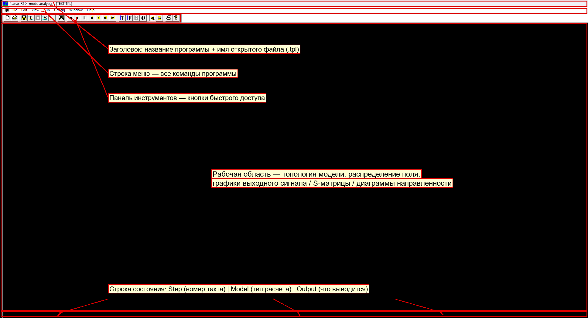
Окно состоит из пяти зон (рамки на рисунке в разделе 1):
| Зона | Назначение |
|---|---|
| Заголовок | Название программы (Planar RT X-mode analyzer) и имя открытого .tpl. |
| Строка меню | Команды: File, Edit, View, Run, Config, Window, Help. |
| Панель инструментов | Кнопки быстрого доступа. |
| Рабочая область | Топология, поле и графики. До команд вывода/расчёта область чёрная. |
| Строка состояния | Step (такт) и Error; Model (тип расчёта); Output (что выводится). |
4. Панель инструментов
Кнопки слева направо (нумерация на рисунке):

| № | Кнопка | Команда (меню) | Горячая клавиша | Что делает |
|---|---|---|---|---|
| 1 |  |
File → New | Ctrl+N |
Создать новый шаблон. |
| 2 | |
File → Open | Ctrl+O |
Открыть .tpl. |
| 3 |  |
Edit → Edit | Alt+F7 |
Открыть .tpl во внешнем редакторе. |
| 4 |  |
View → Output | Alt+Shift+F4 |
Показать выходной сигнал. |
| 5 |  |
View → Field and topology | — | Показать поле с топологией. |
| 6 |  |
View → S-matrix | Ctrl+Shift+F4 |
Показать S-матрицу. |
| 7 |  |
View → Directional Pattern | Ctrl+Alt+F4 |
Показать диаграмму направленности. |
| 8 |  |
View → Statistics | Shift+F4 |
Окно статистики (раздел 6). |
| 9 |  |
Run → Load first step | Shift+F5 |
Вернуться к первому шагу. |
| 10 |  |
Run → Run | F5 |
Расчёт до конца. |
| 11 |  |
Run → Stop | Alt+F5 |
Остановить расчёт. |
| 12 |  |
Run → Run Step | F8 |
Один шаг расчёта. |
| 13 |  |
Run → Load Step | Shift+F8 |
Перечитать текущий шаг. |
| 14 |  |
Run → Skip Step | Ctrl+F6 |
Пропустить шаг вперёд. |
| 15 |  |
Run → Back Step | Alt+F6 |
Шаг назад. |
| 16 |  |
Config → Topology | F4 |
Вывести топологию. |
| 17 |  |
Config → Field | Ctrl+F4 |
Вывести поле. |
| 18 |  |
Config → Synchronization | — | Недоступно (значок серый). |
| 19 |  |
Config → Directional Pattern | — | Настройка/вывод ДН. |
| 20 |  |
Config → Sound | — | Звук (вкл./выкл., мелодия). |
| 21 |  |
Config → AutoRun | — | Автозапуск расчёта. |
| 22 |  |
File → Print | Ctrl+P |
Печать изображения. |
| 23 |  |
Help → About | — | О программе. |
5. Меню
5.1. File (Файл)
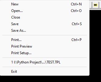
New (Ctrl+N), Open… (Ctrl+O), Close, Save (Ctrl+S), Save As…, Print… (Ctrl+P), Print Preview,
Print Setup…, список недавних файлов, Exit. Назначение — как в любой Windows-программе (создать / открыть /
сохранить / печатать / выйти).
5.2. Edit (Правка)
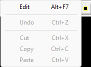
- Edit (
Alt+F7) — открыть текущий.tplво внешнем редакторе (задаётся вConfig → Editor). - Undo / Cut / Copy / Paste — стандартные команды буфера обмена (в текущем режиме недоступны — серые).
5.3. View (Вид)
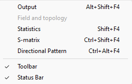
| Пункт | Перевод | Клавиша | Действие |
|---|---|---|---|
| Output | Выходной сигнал | Alt+Shift+F4 |
Показать выходной сигнал. |
| Field and topology | Поле и топология | — | Показать поле с топологией. |
| Statistics | Статистика | Shift+F4 |
Окно статистики (раздел 6). |
| S-matrix | S-матрица | Ctrl+Shift+F4 |
Показать S-матрицу. |
| Directional Pattern | Диаграмма направленности | Ctrl+Alt+F4 |
Показать ДН. В X-моде накопление данных для ДН в текущей версии отключено (см. раздел 7). |
| Toolbar | Панель инструментов | — | Показать/скрыть панель (галочка = показана). |
| Status Bar | Строка состояния | — | Показать/скрыть строку состояния. |
5.4. Run (Расчёт)
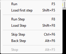
Run (F5), Load first step (Shift+F5), Run Step (F8), Load Step (Shift+F8), Skip Step (Ctrl+F6),
Back Step (Alt+F6), Stop (Alt+F5). Управление расчётом: запуск целиком, по шагам, навигация по тактам,
остановка. (Stop активна только во время счёта.)
5.5. Config (Настройки)
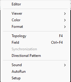
| Пункт | Перевод | Клавиша | Действие |
|---|---|---|---|
| Editor | Редактор | — | Указать внешний редактор для .tpl. |
| Viewer ► | Вьюверы | — | Выбор внешних вьюверов (подменю). |
| Color ► | Цвет | — | Настройка цвета (подменю). |
| Format ► | Формат | — | Формат выходных файлов (подменю). |
| Topology | Топология | F4 |
Вывести топологию. |
| Field | Поле | Ctrl+F4 |
Вывести поле. |
| Synchronization | Синхронизация | — | Недоступно (серый). |
| Directional Pattern | Диаграмма направленности | — | Настройка/вывод ДН. |
| Sound ► | Звук | — | Звуковое сопровождение (подменю). |
| AutoRun | Автозапуск | — | Автоматический запуск расчёта. |
| Setup | Настройка | — | Общие настройки. |
Подменю Config → Viewer — выбор внешних программ просмотра:
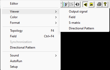
Output signal (TMCROS), Field (FieldView), S-matrix (TMCGROUT), Directional Pattern (TMC_DN).
Подменю Config → Color — BackGround (цвет фона рабочей области):
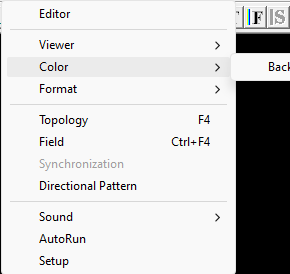
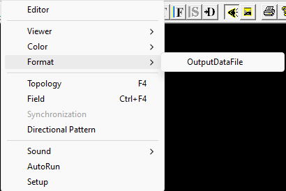
Подменю Config → Format — OutputDataFile (формат/точность чисел выходного файла):
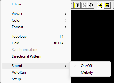
Подменю Config → Sound — On/Off (галочка = включён) и Melody:
5.6. Window (Окно)
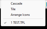
Cascade (каскадом), Tile (мозаикой), Arrange Icons (упорядочить значки), список открытых документов (галочка — активный).
5.7. Help (Справка)

About PlanRT_X… — сведения о версии программы.
6. Диалоговые окна
6.1. About (О программе)
Help → About PlanRT_X… или кнопка . Показывает версию
и сведения о разработчике.
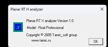
Примечание: в заголовке окна About может стоять надпись «Planar RT H analyzer» (общий с H-ядром ресурс), но текст внутри ясно указывает: Planar RT X analyzer.
6.2. Statistics (Статистика расчёта)
View → Statistics (Shift+F4) или кнопка .
Окно показывает параметры сетки и расчёта.
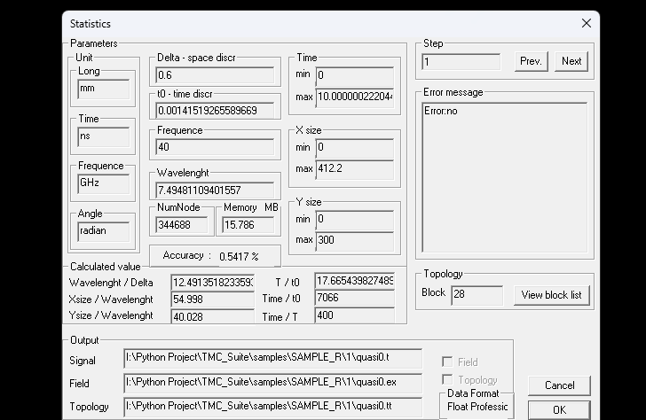
Поля те же, что и в H-ядре:
- Unit — единицы:
Long,Time,Frequence,Angle. - Delta - space discr / t0 - time discr — шаги по пространству и времени.
- Frequence, Wavelenght — частота и длина волны.
- NumNode, Memory MB — число узлов и память.
- Time / X size / Y size (min/max) — интервалы расчёта и размеры области.
- Accuracy — оценка точности.
- Calculated value — производные отношения (
lenght/Delta,Xsize/Wavelenght,T/t0и т. д.). - Step + кнопки Prev. / Next — навигация по шагам.
- Error message — сообщение об ошибке (
Error:no— ошибок нет). - Topology → Block + View block list — блоки модели.
- Output — пути к выходным файлам, флажки Field / Topology, Data Format.
- Кнопки OK / Cancel.
7. Чем X-мода отличается от H (для пользователя)
Для пользователя интерфейс и формат данных одинаковы с H-ядром. Различается то, что считается «под капотом»:
| Свойство | H-ядро | X-ядро |
|---|---|---|
| Цикл расчёта (1T) | 2 подтакта | 4 подтакта |
| Компонент поля на узле | 4 | 8 |
| Доп. типы блоков топологии | — | RECT_STAT_Y, CIRCLE_STAT_Y, POLYGON_STAT_Y, FILE_Y |
| Диаграмма направленности | накапливается | в текущей версии накопление отключено |
| Сигнатура входного файла | #TMC_RT_H |
#TMC_RT_H (та же) |
Практические следствия:
- Формат
.tpl— тот же, и первая строка файла остаётся#TMC_RT_H(отдельной сигнатуры#TMC_RT_Xнет). Поэтому один и тот же шаблон можно открыть и H-, и X-ядром. - X-ядро дополнительно понимает в секции
#TOPOLOGYблоки с суффиксом_Y(RECT_STAT_Yи т. д.). - Из-за большего числа компонент поля X-расчёт требует больше памяти и времени при той же сетке —
следите за
NumNodeиMemoryв окне статистики. - Пункт View → Directional Pattern в X-моде может не давать результата, так как накопление данных для ДН в текущей версии отключено.
Только для сборки (не для пользователя готовой программы). X-ядро компилируется с шестью препроцессорными макросами (
ELECTRON_Q___,ELECTRON_M___,CTMCRTH_INDANBLCK_FILEY,CTMCRTH_INDANBLCK_RECTSTATY,CTMCRTH_INDANBLCK_CIRCSTATY,CTMCRTH_INDANBLCK_POLYGSTTY), которые задаются только в свойствах проекта X-моды. На работу с уже готовымtmc_rtx.exeэто никак не влияет — подробности вdocs/build-guide/иdocs/api/kernels/planar_rt_x.md.
8. Входные данные: файл-шаблон .tpl
8.1. Расширение и общая идея
Главный входной файл — текстовый шаблон .tpl. Первая строка — сигнатура #TMC_RT_H. Перед
расчётом файл проходит препроцессинг библиотекой PREPR (#include, #define, вычисление выражений).
Структура файла полностью совпадает с H-ядром (исчерпывающий разбор — в planar_rt_h.md, раздел 7);
ниже приведён собственный учебный пример X-ядра.
Спецсимволы:
- # в начале строки — директива препроцессора (#include, #define, #STEP, #EOF);
- ! в начале строки — комментарий (поясняющий текст, игнорируется);
- ; — разделитель параметров;
- \\ в конце строки — перенос длинной строки.
8.2. Разбор учебного примера 1.TPL
Файл src/kernels/PlanarRT_X/1.TPL снабжён подробными комментариями и показывает почти все возможности
формата (это справочный пример синтаксиса; для запуска ему нужен подключаемый planrt2.h). Его структура:
#TMC_RT_H              ← сигнатура
#include planrt2.h     ← подключаемые константы

#STEP                  ← первый шаг расчёта
  #PARM … #END_PARM        — параметры
  #TOPOLOGY … #END_TOPOLOGY — геометрия (блоки)
  #LINK_LIST … #END_LINK    — размещение блоков
  #OUTPUT … #END_OUTPUT     — выходные файлы
#END_STEP

#STEP … #END_STEP      ← второй шаг (можно несколько)

#EOF                   ← конец файла
Файл может содержать несколько секций #STEP — это последовательность расчётов (например, разные
конфигурации топологии), переключаемых кнопками Prev./Next в окне статистики и командами меню Run.
8.3. Секция #PARM (параметры)
 ANGLE_UNIT radian;     ! единица углов
 FREQ_UNIT GHz;         ! единица частоты
 LONG_UNIT mm;          ! единица длины
 TIME_UNIT s;           ! единица времени
 DELTA 0.35;            ! шаг сетки Δ
 TIME -.0001; 0.0001;   ! интервал времени (от; до)
 X_MIN -10.0*2-4 ;      ! границы по X (можно выражением)
 X_MAX ( + 500 . 0 ) ;
 Y_MIN (-5.0);          ! границы по Y
 Y_MAX 300.0;
 FREQ 40.0;             ! рабочая частота
Числа можно задавать выражениями; пробелы внутри чисел/скобок допускаются (( + 500 . 0 ) = 500.0).
8.4. Секция #TOPOLOGY (геометрия)
Геометрия описывается блоками BLOCK n; … END_B. Внутри блока — один элемент. Типы элементов
(из комментариев примера):
| Ключевое слово | Синтаксис | Что задаёт |
|---|---|---|
RECT_STAT |
RECT_STAT E(x,y); x_min; x_max; y_min; y_max; |
Неподвижный прямоугольник; E(x,y) — материал или выражение. |
CIRCLE_STAT |
CIRCLE_STAT E(r,f); r_min; r_max; f_min; f_max; |
Неподвижный круговой сегмент (диапазоны радиуса r и угла f). |
POLYGON_STAT |
POLYGON_STAT E(x,y); L x; y; … |
Неподвижный многоугольник; вершины строками L x; y;. |
RECT_MOVE |
RECT_MOVE E(x,y); x_min; x_max; y_min; y_max; Vx; Vy; w; |
Подвижный прямоугольник со скоростями Vx,Vy и угловой скоростью w. |
CIRCLE_MOVE |
CIRCLE_MOVE E(r,f); r_min; r_max; f_min; f_max; Vx; Vy; w; |
Подвижный круговой сегмент. |
POLYGON_MOVE |
POLYGON_MOVE E(x,y); Vx; Vy; w; L x; y; … |
Подвижный многоугольник. |
INPUT_X |
INPUT_X <тип>; y_min; y_max; t_min; t_max; [Amp]; [Faza]; [Eps]; |
Вход вдоль оси Y — на левой или правой границе «коробки», размеры по Y в диапазоне y_min…y_max, радиоимпульс во времени t_min…t_max. |
INPUT_Y |
INPUT_Y <тип>; x_min; x_max; t_min; t_max; [Amp]; [Faza]; [Eps]; |
Вход вдоль оси X — на нижней или верхней границе, размеры по X. |
E(x,y) — это «материал» элемента; может быть:
- ключевым словом METAL (идеальный проводник), MAGNETIC (магнетик — стенка холостого
хода) или ABSORBER (поглотитель);
- выражением для неоднородной среды, например - ( x^2 + y^2 ) или - ( 3 - r ) (распределение ε как
функция координат).
Выражение задаёт добавку ε⁺ к проницаемости вакуума, а не саму ε. Среде с ε = 4 соответствует запись
3, вакууму —0, среде с ε = 0 —-1.Первый параметр входа — это мода, а не форма сигнала.
MAGNETIC— плоская волна (ширина входа меньше половины длины волны);METALили пусто — волна H₁₀ прямоугольного волновода (ширина больше половины, но меньше полной длины волны). Амплитуда и фаза задаются необязательными параметрами 6 и 7 как выражения отtиf; параметр 8 — добавка ε в сечении входа. Подробно — вtpl-guide.md, раздел 5.5.
Полное описание всех примитивов, включая плазменные варианты RECT_STAT_N / _B / _Y, — в
tpl-guide.md.
Пример блока с поясняющими комментариями (как в файле):
 BLOCK 1;
! прямоугольник, заполненный распределением ε = -(x²+y²)
! RECT_STAT E(x,y); x_min; x_max; y_min; y_max;
 RECT_STAT - ( x^2 + y^2 ) ; -1 ; 3 ; -2; 4;
 END_B
Подвижный элемент добавляет три числа в конце — скорости Vx, Vy (в LONG_UNIT/TIME_UNIT) и угловую
скорость w (в ANGLE_UNIT/TIME_UNIT):
 BLOCK 3;
! подвижный прямоугольник со скоростью (Vx,Vy) и вращением w
 RECT_MOVE - ( x^2 + y^2 ) ; -1; 3; -2; 4; 1.0; -2; 10;
 END_B
8.5. Секция #LINK_LIST (размещение блоков)
! блок n размещается в точке (x0, y0); координаты в единицах из #PARM
! T n; x0; y0;
 T 1; -1.0; -0.5;
 T 2; -1.0; -0.5;
 ...
Каждая строка T <номер блока>; x0; y0; ставит блок в координаты (x0, y0) общей расчётной области.
То есть в #TOPOLOGY форма блока задаётся «локально», а в #LINK_LIST — где он стоит.
8.6. Секция #OUTPUT (выходные файлы)
 FILE out1;     ! базовое имя выходных файлов
 FIELDS;        ! сохранять распределение поля
 TOPOLOGY;      ! сохранять топологию
| Команда | Назначение |
|---|---|
FILE <имя>; |
Базовое имя для выходных файлов. Обязательна, должна быть первой; имя не должно содержать точку. |
SMATRIX <Sfile>; <частота>; <T_min>; <T_max>; |
Записать S-матрицу в Sfile.s для указанной частоты, усреднив по интервалу T_min…T_max. |
FIELDS; |
Сохранять распределение поля (.ex и др.). Требует также TOPOLOGY;. Сильно замедляет счёт. |
TOPOLOGY; |
Сохранять топологию (.tt). |
FIELD_DISTRIBUTION <имя>; <частота>; <expr>; <expr>; |
Комплексное распределение поля (модуль → .em, фаза → .ef). |
FIELD_DISTRIBUTION_M <имя>; <частота>; <expr>; <expr>; |
То же, вариант с накоплением в памяти. |
Во втором шаге примера эти строки закомментированы (! TOPOLOGY, ! FIELD) — значит, для второго шага
поле и топология не выводятся.
8.7. Как подготовить свои данные
- Скопируйте пример
1.TPL(и подключаемыйplanrt2.h) в отдельную папку. - В секции
#PARMзадайте единицы, шагDELTA, интервалTIME, границы области и частоту. - Опишите геометрию в
#TOPOLOGY(блокиBLOCK … END_B), при необходимости используйте подвижные элементы*_MOVEи входыINPUT_X/INPUT_Y. - Разместите блоки в
#LINK_LIST(T n; x0; y0;). - В
#OUTPUTзадайте имя выходных файлов и что сохранять. - Откройте
.tplв программе и запустите расчёт.
9. Выходные данные
| Расширение | Содержимое | Чем смотреть |
|---|---|---|
.t |
Временно́й сигнал на входах | TMCROS |
.s |
S-матрица рассеяния | TMCGROUT |
.ex |
Распределение поля Ex (двоичный) | FieldView |
.ey, .hz |
Распределение полей Ey, Hz | FieldView |
.em, .ef |
Модуль и фаза комплексного распределения поля | FieldView |
.q, .ix, .iy |
Служебные файлы | — |
.tt |
Топология модели | FieldView |
.eps |
Распределение ε | ядро (вход и выход) |
10. Типовые сценарии
Открыть расчёт и посмотреть результат:
1. File → Open… → выбрать .tpl.
2. Config → Topology (F4) — проверить топологию.
3. Run → Run (F5) — выполнить расчёт.
4. View → Output / View → S-matrix — посмотреть результаты.
Пошаговый расчёт с наблюдением поля:
1. Run → Load first step (Shift+F5).
2. Run → Run Step (F8) — по одному шагу.
3. Config → Field (Ctrl+F4) — наблюдать поле.
Многошаговый шаблон: если в файле несколько #STEP, переключайтесь между ними кнопками
Prev./Next в окне статистики.
Проверка ресурсов: View → Statistics (Shift+F4) — узлы, память, точность (для X-моды особенно
важно из-за повышенного расхода памяти).
11. Возможные проблемы
| Симптом | Что проверить |
|---|---|
| Файл не открывается | Первая строка — #TMC_RT_H; рядом лежат все #include-файлы. |
| Рабочая область чёрная | Выполните Config → Topology (F4) или запустите расчёт. |
Edit → Edit не работает |
Сначала задайте редактор в Config → Editor. |
Error ≠ no в строке состояния |
Посмотрите Error message в окне статистики. |
View → Directional Pattern пуст |
В X-моде накопление данных для ДН отключено (раздел 7). |
| Нехватка памяти / медленно | X-мода расходует больше ресурсов; увеличьте DELTA или уменьшите область. |
12. Связанные программы и документы
- PlanarRT_H — парное ядро (H-поляризация). См.
planar_rt_h.md(там же исчерпывающий разбор формата.tpl). - TMCROS (
.t), TMCGROUT (.s), TMC_DN (ДН), FieldView (.ex,.tt) — вьюверы. - API-документация:
docs/api/kernels/planar_rt_x.md; формат данных:docs/api/libs/tmcindan.md.
User manual — the PlanarRT_X compute kernel (tmc_rtx.exe)
Program: Planar RT X-mode analyzer (the executable
tmc_rtx.exe). The program's interface is in English — the English item names are given as in the program, with an explanation next to them. The captions on the screenshots are in Russian.PlanarRT_X is the "companion" program to PlanarRT_H. Both are built from the same source code, so their interface (menu, toolbar, dialogs) is completely identical. Only the physics of the computation differs: H computes H-polarization, X computes the X-mode (see section 7). If you are already familiar with
planar_rt_h.md, mastering X will be easy. Below is the full description with screenshots of the X program specifically.
1. Purpose of the program
PlanarRT_X is a compute kernel of the TMC Suite package for the
electrodynamic computation of planar (two-dimensional) structures in the
X-mode in the time domain. Like the H kernel, from a text template .tpl
(the area topology, parameters, output data) the program "plays" the field over
time and saves the results for viewing in the viewers:
- the time signal at the inputs (
.t) → the TMCROS viewer; - the scattering S-matrix (
.s) → the TMCGROUT viewer; - the field distribution (
.ex,.ey,.hz,.em,.ef) and the topology (.tt) → the FieldView viewer.
The main difference from the H kernel is the internal algorithm: in the X-mode more field components are stored at each grid node, and the computation cycle consists of four sub-steps instead of two (details in section 7).
2. Launching the program and opening data
- Launch the file
tmc_rtx.exe(folderdist/win32/bin/). The main window opens. - Open a template: File → Open… (or the
button, or
Ctrl+O). - Choose a file with the
.tplextension. The filesamples/SAMPLE_R/1/TEST.TPLworks as a starting sample (it opens in both the H and X kernels). - The file name appears in the title:
Planar RT X-mode analyzer - [TEST.TPL].
For studying the format the file
src/kernels/PlanarRT_X/1.TPLis convenient — it is provided with detailed comments for all block types (see section 8.2). Note: to actually run it, the fileplanrt2.hit includes must be next to it; if that file is missing, use a ready sample for the computation (for example,TEST.TPL), and read1.TPLas a syntax reference.You can launch with a file from the command line:
tmc_rtx.exe
"path\to\file.tpl"
.
3. The main window
The window consists of five zones (frames in the figure in section 1):
| Zone | Purpose |
|---|---|
| Title bar | The program name (Planar RT X-mode analyzer) and the name of the open .tpl. |
| Menu bar | Commands: File, Edit, View, Run, Config, Window, Help. |
| Toolbar | Quick-access buttons. |
| Work area | Topology, field and graphs. Before output/computation commands the area is black. |
| Status bar | Step (the step) and Error; Model (computation type); Output (what is output). |
4. The toolbar
The buttons from left to right (numbered in the figure):
| # | Button | Command (menu) | Shortcut | What it does |
|---|---|---|---|---|
| 1 | |
File → New | Ctrl+N |
Create a new template. |
| 2 | |
File → Open | Ctrl+O |
Open a .tpl. |
| 3 | |
Edit → Edit | Alt+F7 |
Open the .tpl in an external editor. |
| 4 | |
View → Output | Alt+Shift+F4 |
Show the output signal. |
| 5 | |
View → Field and topology | — | Show the field with the topology. |
| 6 | |
View → S-matrix | Ctrl+Shift+F4 |
Show the S-matrix. |
| 7 | |
View → Directional Pattern | Ctrl+Alt+F4 |
Show the radiation pattern. |
| 8 | |
View → Statistics | Shift+F4 |
The statistics window (section 6). |
| 9 | |
Run → Load first step | Shift+F5 |
Return to the first step. |
| 10 | |
Run → Run | F5 |
Compute to the end. |
| 11 | |
Run → Stop | Alt+F5 |
Stop the computation. |
| 12 | |
Run → Run Step | F8 |
One computation step. |
| 13 | |
Run → Load Step | Shift+F8 |
Re-read the current step. |
| 14 | |
Run → Skip Step | Ctrl+F6 |
Skip one step forward. |
| 15 | |
Run → Back Step | Alt+F6 |
One step back. |
| 16 | |
Config → Topology | F4 |
Output the topology. |
| 17 | |
Config → Field | Ctrl+F4 |
Output the field. |
| 18 | |
Config → Synchronization | — | Unavailable (the icon is gray). |
| 19 | |
Config → Directional Pattern | — | Configure/output the pattern. |
| 20 | |
Config → Sound | — | Sound (on/off, melody). |
| 21 | |
Config → AutoRun | — | Automatic start of the computation. |
| 22 | |
File → Print | Ctrl+P |
Print the image. |
| 23 | |
Help → About | — | About the program. |
5. The menus
5.1. File
New (Ctrl+N), Open… (Ctrl+O), Close, Save (Ctrl+S), Save As…, Print…
(Ctrl+P), Print Preview, Print Setup…, the recent files list, Exit. Their
purpose is as in any Windows program (create / open / save / print / exit).
5.2. Edit
- Edit (
Alt+F7) — open the current.tplin the external editor (set inConfig → Editor). - Undo / Cut / Copy / Paste — standard clipboard commands (unavailable in the current mode — gray).
5.3. View
| Item | Translation | Shortcut | Action |
|---|---|---|---|
| Output | Output signal | Alt+Shift+F4 |
Show the output signal. |
| Field and topology | Field and topology | — | Show the field with the topology. |
| Statistics | Statistics | Shift+F4 |
The statistics window (section 6). |
| S-matrix | S-matrix | Ctrl+Shift+F4 |
Show the S-matrix. |
| Directional Pattern | Radiation pattern | Ctrl+Alt+F4 |
Show the pattern. In the X-mode the accumulation of pattern data is disabled in the current version (see section 7). |
| Toolbar | Toolbar | — | Show/hide the toolbar (a check mark = shown). |
| Status Bar | Status bar | — | Show/hide the status bar. |
5.4. Run
Run (F5), Load first step (Shift+F5), Run Step (F8), Load Step (Shift+F8),
Skip Step (Ctrl+F6), Back Step (Alt+F6), Stop (Alt+F5). Computation control:
run in full, step by step, navigation through steps, stop. (Stop is active only
during a computation.)
5.5. Config
| Item | Translation | Shortcut | Action |
|---|---|---|---|
| Editor | Editor | — | Specify the external editor for .tpl. |
| Viewer ► | Viewers | — | Choose external viewers (submenu). |
| Color ► | Color | — | Color settings (submenu). |
| Format ► | Format | — | Output-file format (submenu). |
| Topology | Topology | F4 |
Output the topology. |
| Field | Field | Ctrl+F4 |
Output the field. |
| Synchronization | Synchronization | — | Unavailable (gray). |
| Directional Pattern | Radiation pattern | — | Configure/output the pattern. |
| Sound ► | Sound | — | Sound accompaniment (submenu). |
| AutoRun | AutoRun | — | Automatic start of the computation. |
| Setup | Setup | — | General settings. |
The Config → Viewer submenu — choosing external viewer programs:
Output signal (TMCROS), Field (FieldView), S-matrix (TMCGROUT), Directional Pattern (TMC_DN).
The Config → Color submenu — BackGround (the background color of the work
area):
The Config → Format submenu — OutputDataFile (the format/precision of the
numbers in the output file):
The Config → Sound submenu — On/Off (a check mark = on) and Melody:
5.6. Window
Cascade, Tile, Arrange Icons, the list of open documents (a check mark — the active one).
5.7. Help
About PlanRT_X… — information about the program version.
6. Dialog windows
6.1. About
Help → About PlanRT_X… or the
button. Shows the version and
developer information.
Note: the About window title may read "Planar RT H analyzer" (a resource shared with the H kernel), but the text inside clearly states: Planar RT X analyzer.
6.2. Statistics
View → Statistics (Shift+F4) or the
button. The window shows the
grid and computation parameters.
The fields are the same as in the H kernel:
- Unit — units:
Long,Time,Frequence,Angle. - Delta - space discr / t0 - time discr — the space and time steps.
- Frequence, Wavelenght — the frequency and wavelength.
- NumNode, Memory MB — the number of nodes and the memory.
- Time / X size / Y size (min/max) — the computation intervals and area sizes.
- Accuracy — an accuracy estimate.
- Calculated value — derived ratios (
lenght/Delta,Xsize/Wavelenght,T/t0, etc.). - Step + the Prev. / Next buttons — step navigation.
- Error message — an error message (
Error:no— no errors). - Topology → Block + View block list — the model blocks.
- Output — the paths to the output files, the Field / Topology checkboxes, Data Format.
- The OK / Cancel buttons.
7. How the X-mode differs from H (for the user)
For the user the interface and the data format are the same as in the H kernel. What differs is what is computed "under the hood":
| Property | H kernel | X kernel |
|---|---|---|
| Computation cycle (1T) | 2 sub-steps | 4 sub-steps |
| Field components per node | 4 | 8 |
| Additional topology block types | — | RECT_STAT_Y, CIRCLE_STAT_Y, POLYGON_STAT_Y, FILE_Y |
| Radiation pattern | accumulated | accumulation disabled in the current version |
| Input-file signature | #TMC_RT_H |
#TMC_RT_H (the same) |
Practical consequences:
- The
.tplformat is the same, and the first line of the file stays#TMC_RT_H(there is no separate#TMC_RT_Xsignature). So the same template can be opened by both the H and X kernels. - The X kernel additionally understands, in the
#TOPOLOGYsection, blocks with the_Ysuffix (RECT_STAT_Y, etc.). - Because of the larger number of field components, an X computation requires
more memory and time for the same grid — watch
NumNodeandMemoryin the statistics window. - The View → Directional Pattern item in the X-mode may give no result, since the accumulation of pattern data is disabled in the current version.
For the build only (not for the user of the finished program). The X kernel is compiled with six preprocessor macros (
ELECTRON_Q___,ELECTRON_M___,CTMCRTH_INDANBLCK_FILEY,CTMCRTH_INDANBLCK_RECTSTATY,CTMCRTH_INDANBLCK_CIRCSTATY,CTMCRTH_INDANBLCK_POLYGSTTY), which are set only in the X-mode project properties. This does not affect working with an already-builttmc_rtx.exein any way — details are indocs/build-guide/anddocs/api/kernels/planar_rt_x.md.
8. Input data: the .tpl template file
8.1. Extension and the general idea
The main input file is a text template .tpl. The first line is the signature
#TMC_RT_H. Before the computation the file goes through preprocessing by the
PREPR library (#include, #define, expression evaluation). The file structure is
completely identical to the H kernel (an exhaustive breakdown is in
planar_rt_h.md, section 7); below is the X kernel's own tutorial example.
Special characters:
- # at the start of a line — a preprocessor directive (#include, #define,
#STEP, #EOF);
- ! at the start of a line — a comment (explanatory text, ignored);
- ; — a parameter separator;
- \\ at the end of a line — a continuation of a long line.
8.2. Walkthrough of the tutorial example 1.TPL
The file src/kernels/PlanarRT_X/1.TPL is provided with detailed comments and
shows almost all the format's capabilities (it is a syntax reference example; to
run it, it needs the included planrt2.h). Its structure:
#TMC_RT_H              ← signature
#include planrt2.h     ← included constants

#STEP                  ← the first computation step
  #PARM … #END_PARM        — parameters
  #TOPOLOGY … #END_TOPOLOGY — geometry (blocks)
  #LINK_LIST … #END_LINK    — block placement
  #OUTPUT … #END_OUTPUT     — output files
#END_STEP

#STEP … #END_STEP      ← the second step (there can be several)

#EOF                   ← end of file
A file may contain several #STEP sections — this is a sequence of
computations (for example, different topology configurations), switched with the
Prev./Next buttons in the statistics window and the Run menu commands.
8.3. The #PARM section (parameters)
 ANGLE_UNIT radian;     ! angle unit
 FREQ_UNIT GHz;         ! frequency unit
 LONG_UNIT mm;          ! length unit
 TIME_UNIT s;           ! time unit
 DELTA 0.35;            ! grid step Δ
 TIME -.0001; 0.0001;   ! time interval (from; to)
 X_MIN -10.0*2-4 ;      ! X boundaries (an expression is allowed)
 X_MAX ( + 500 . 0 ) ;
 Y_MIN (-5.0);          ! Y boundaries
 Y_MAX 300.0;
 FREQ 40.0;             ! operating frequency
Numbers can be given as expressions; spaces inside numbers/parentheses are allowed
(( + 500 . 0 ) = 500.0).
8.4. The #TOPOLOGY section (geometry)
The geometry is described by blocks BLOCK n; … END_B. Inside a block there is
one element. Element types (from the example's comments):
| Keyword | Syntax | What it sets |
|---|---|---|
RECT_STAT |
RECT_STAT E(x,y); x_min; x_max; y_min; y_max; |
A stationary rectangle; E(x,y) is the material or an expression. |
CIRCLE_STAT |
CIRCLE_STAT E(r,f); r_min; r_max; f_min; f_max; |
A stationary circular segment (ranges of radius r and angle f). |
POLYGON_STAT |
POLYGON_STAT E(x,y); L x; y; … |
A stationary polygon; vertices by L x; y; lines. |
RECT_MOVE |
RECT_MOVE E(x,y); x_min; x_max; y_min; y_max; Vx; Vy; w; |
A moving rectangle with velocities Vx,Vy and angular velocity w. |
CIRCLE_MOVE |
CIRCLE_MOVE E(r,f); r_min; r_max; f_min; f_max; Vx; Vy; w; |
A moving circular segment. |
POLYGON_MOVE |
POLYGON_MOVE E(x,y); Vx; Vy; w; L x; y; … |
A moving polygon. |
INPUT_X |
INPUT_X <type>; y_min; y_max; t_min; t_max; [Amp]; [Faza]; [Eps]; |
An input along the Y axis — on the left or right boundary of the "box"; its extent is given along Y in the range y_min…y_max, with a radio pulse in time t_min…t_max. |
INPUT_Y |
INPUT_Y <type>; x_min; x_max; t_min; t_max; [Amp]; [Faza]; [Eps]; |
An input along the X axis — on the bottom or top boundary; its extent is given along X. |
E(x,y) is the "material" of the element; it can be:
- the keyword METAL (a perfect conductor), MAGNETIC (a magnetic — an
open-circuit wall) or ABSORBER (an absorber);
- an expression for an inhomogeneous medium, for example - ( x^2 + y^2 ) or
- ( 3 - r ) (the ε distribution as a function of coordinates).
An expression sets the addition ε⁺ to the permittivity of vacuum, not ε itself. A medium with ε = 4 corresponds to writing
3, vacuum to0, and a medium with ε = 0 to-1.The first parameter of an input is the mode, not the signal shape.
MAGNETIC— a plane wave (the input is narrower than half a wavelength);METALor empty — the H₁₀ wave of a rectangular waveguide (wider than half but narrower than a full wavelength). The amplitude and phase are given by the optional parameters 6 and 7 as expressions intandf; parameter 8 is the ε addition in the cross-section of the input. Seetpl-guide.md, section 5.5, for details.
The full description of all primitives, including the plasma variants
RECT_STAT_N / _B / _Y, is in tpl-guide.md.
An example block with explanatory comments (as in the file):
 BLOCK 1;
! a rectangle filled with the distribution ε = -(x²+y²)
! RECT_STAT E(x,y); x_min; x_max; y_min; y_max;
 RECT_STAT - ( x^2 + y^2 ) ; -1 ; 3 ; -2; 4;
 END_B
A moving element adds three numbers at the end — the velocities Vx, Vy (in
LONG_UNIT/TIME_UNIT) and the angular velocity w (in ANGLE_UNIT/TIME_UNIT):
 BLOCK 3;
! a moving rectangle with velocity (Vx,Vy) and rotation w
 RECT_MOVE - ( x^2 + y^2 ) ; -1; 3; -2; 4; 1.0; -2; 10;
 END_B
The X kernel additionally recognizes blocks with the
_Ysuffix (RECT_STAT_Y,CIRCLE_STAT_Y,POLYGON_STAT_Y,FILE_Y).
8.5. The #LINK_LIST section (block placement)
! block n is placed at the point (x0, y0); coordinates in the units from #PARM
! T n; x0; y0;
 T 1; -1.0; -0.5;
 T 2; -1.0; -0.5;
 ...
Each line T <block number>; x0; y0; places the block at the coordinates (x0,
y0) of the common computation area. That is, in #TOPOLOGY the shape of a block
is set "locally", and in #LINK_LIST — where it stands.
8.6. The #OUTPUT section (output files)
 FILE out1;     ! base name of the output files
 FIELDS;        ! save the field distribution
 TOPOLOGY;      ! save the topology
| Command | Purpose |
|---|---|
FILE <name>; |
The base name for the output files. Mandatory, must come first; the name must not contain a dot. |
SMATRIX <Sfile>; <frequency>; <T_min>; <T_max>; |
Write the S-matrix into Sfile.s for the given frequency, averaged over the interval T_min…T_max. |
FIELDS; |
Save the field distribution (.ex and others). Also requires TOPOLOGY;. Slows the computation down considerably. |
TOPOLOGY; |
Save the topology (.tt). |
FIELD_DISTRIBUTION <name>; <frequency>; <expr>; <expr>; |
The complex field distribution (magnitude → .em, phase → .ef). |
FIELD_DISTRIBUTION_M <name>; <frequency>; <expr>; <expr>; |
The same, the variant that accumulates in memory. |
In the second step of the example these lines are commented out (! TOPOLOGY, !
FIELD) — meaning that for the second step the field and topology are not output.
8.7. How to prepare your own data
- Copy the example
1.TPL(and the includedplanrt2.h) into a separate folder. - In the
#PARMsection set the units, theDELTAstep, theTIMEinterval, the area boundaries and the frequency. - Describe the geometry in
#TOPOLOGY(theBLOCK … END_Bblocks), using the moving elements*_MOVEand the inputsINPUT_X/INPUT_Yif needed. - Place the blocks in
#LINK_LIST(T n; x0; y0;). - In
#OUTPUTset the output file name and what to save. - Open the
.tplin the program and run the computation.
9. Output data
| Extension | Contents | What to view it with |
|---|---|---|
.t |
The time signal at the inputs | TMCROS |
.s |
The scattering S-matrix | TMCGROUT |
.ex |
The Ex field distribution (binary) | FieldView |
.ey, .hz |
The Ey, Hz field distributions | FieldView |
.em, .ef |
The magnitude and phase of the complex field distribution | FieldView |
.q, .ix, .iy |
Service files | — |
.tt |
The model topology | FieldView |
.eps |
The ε distribution | the kernel (input and output) |
10. Typical scenarios
Open a computation and view the result:
1. File → Open… → select a .tpl.
2. Config → Topology (F4) — check the topology.
3. Run → Run (F5) — perform the computation.
4. View → Output / View → S-matrix — view the results.
Step-by-step computation with field observation:
1. Run → Load first step (Shift+F5).
2. Run → Run Step (F8) — one step at a time.
3. Config → Field (Ctrl+F4) — observe the field.
Multi-step template: if the file has several #STEP, switch between them with
the Prev./Next buttons in the statistics window.
Resource check: View → Statistics (Shift+F4) — nodes, memory, accuracy
(especially important for the X-mode because of the increased memory consumption).
11. Possible problems
| Symptom | What to check |
|---|---|
| The file does not open | The first line is #TMC_RT_H; all #include files are next to it. |
| The work area is black | Run Config → Topology (F4) or start the computation. |
Edit → Edit does not work |
First set the editor in Config → Editor. |
Error ≠ no in the status bar |
Look at the Error message in the statistics window. |
View → Directional Pattern is empty |
In the X-mode the accumulation of pattern data is disabled (section 7). |
| Not enough memory / slow | The X-mode consumes more resources; increase DELTA or reduce the area. |
12. Related programs and documents
- PlanarRT_H — the companion kernel (H-polarization). See
planar_rt_h.md(which also has the exhaustive breakdown of the.tplformat). - TMCROS (
.t), TMCGROUT (.s), TMC_DN (pattern), FieldView (.ex,.tt) — the viewers. - API documentation:
docs/api/kernels/planar_rt_x.md; the data format:docs/api/libs/tmcindan.md.