Руководство пользователя — счётное ядро PlanarRT_H (tmc_rth.exe)
Программа: Planar RT H analyzer (исполняемый файл
tmc_rth.exe). Интерфейс программы англоязычный — в руководстве приводятся английские названия пунктов как в программе, а рядом — русское пояснение. Подписи на скриншотах русские.
1. Назначение программы
PlanarRT_H — это счётное ядро пакета TMC Suite. Оно выполняет электродинамический расчёт планарных (двумерных) структур в поляризации H во временно́й области: по заданной топологии (металл, поглотители, диэлектрики, входы) программа шаг за шагом вычисляет, как распространяется и рассеивается электромагнитное поле.
Простыми словами: вы описываете «карту» расчётной области в текстовом файле-шаблоне .tpl, а ядро
«проигрывает» по ней волну во времени и сохраняет результаты:
- временно́й сигнал на входах (
.t) — его потом смотрят во вьювере TMCROS; - S-матрицу рассеяния (
.s) — её смотрят во вьювере TMCGROUT; - распределение поля (
.ex,.ey,.hz,.em,.ef) и топологию (.tt) — их смотрят во вьювере FieldView.
Таким образом, PlanarRT_H — это «генератор данных»: он считает, а отдельные программы-вьюверы рисуют
результат. (Парное ядро PlanarRT_X делает то же самое для X-моды — см. planar_rt_x.md.)
2. Запуск программы и открытие данных
- Запустите файл
tmc_rth.exe(папкаdist/win32/bin/). Откроется главное окно (см. рисунок выше). - Откройте файл-шаблон расчёта: меню File → Open… (или кнопка
 на панели инструментов, или
 Ctrl+O). - В диалоге выбора файла укажите файл с расширением
.tpl(например,samples/SAMPLE_R/1/TEST.TPL). - После открытия имя файла появится в заголовке окна:
Planar RT H analyzer - [TEST.TPL].
Можно также запустить программу сразу с файлом, перетащив
.tplна значок программы или указав путь к файлу аргументом командной строки:tmc_rth.exe "путь\к\файлу.tpl".
3. Главное окно
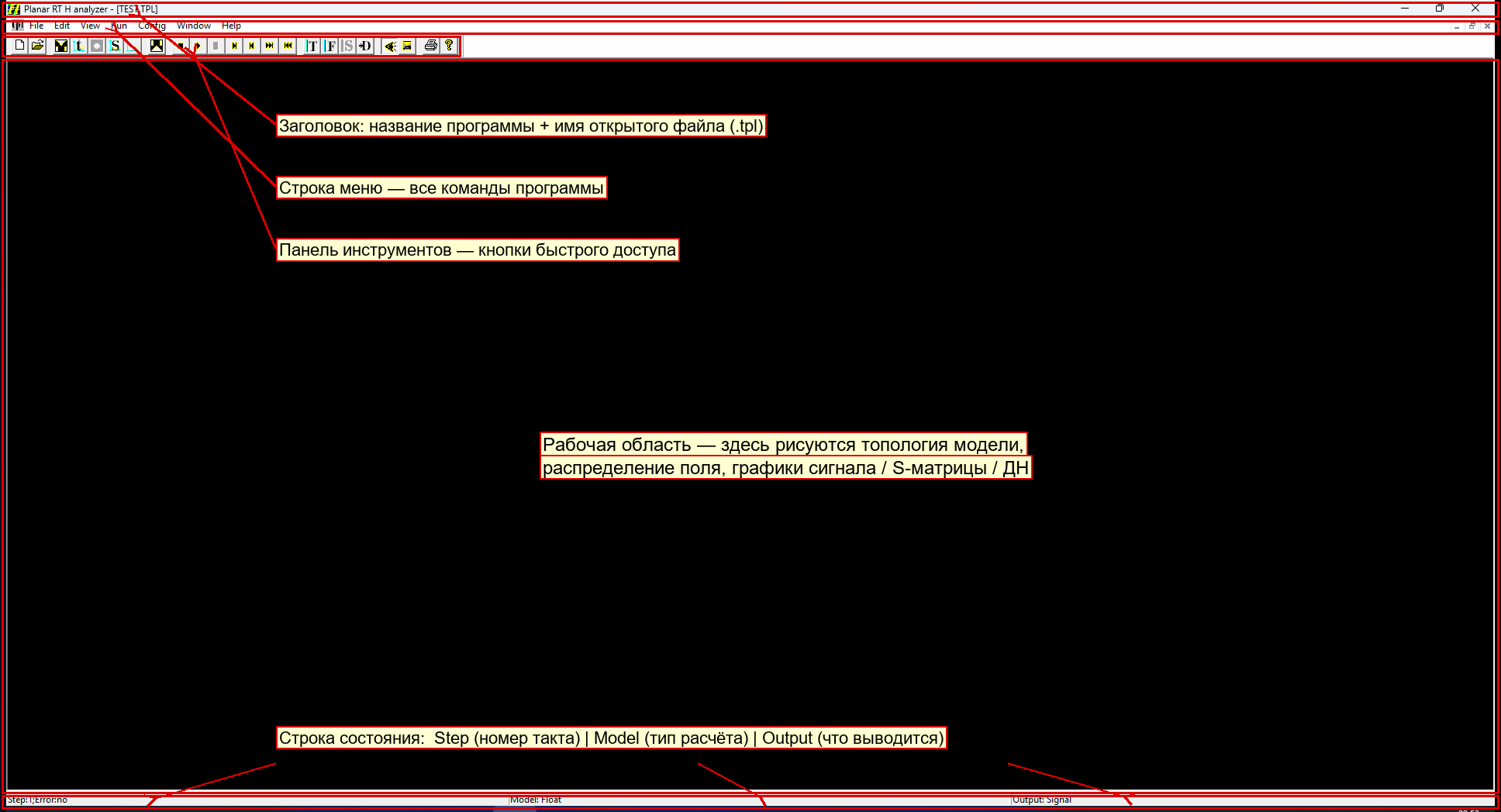
Главное окно состоит из пяти зон (показаны рамками на рисунке в разделе 1):
| Зона | Назначение |
|---|---|
| Заголовок | Название программы и имя открытого файла .tpl. |
| Строка меню | Все команды программы: File, Edit, View, Run, Config, Window, Help. |
| Панель инструментов | Кнопки быстрого доступа к самым частым командам. |
| Рабочая область | Здесь рисуются топология модели, распределение поля и графики (сигнал / S-матрица / ДН). Сразу после открытия файла область чёрная — изображение появляется после команд вывода или расчёта. |
| Строка состояния | Слева — Step (номер текущего такта расчёта) и признак ошибки Error; по центру — Model (тип/точность расчёта: Double при двойной точности, Float при одинарной; в текущей сборке — Double); справа — Output (что выводится, например Signal). |
4. Панель инструментов
Панель инструментов дублирует самые нужные пункты меню. Кнопки слева направо пронумерованы:

| № | Кнопка | Команда (меню) | Горячая клавиша | Что делает |
|---|---|---|---|---|
| 1 |  |
File → New | Ctrl+N |
Создать новый (пустой) шаблон. |
| 2 | |
File → Open | Ctrl+O |
Открыть существующий .tpl-файл. |
| 3 |  |
Edit → Edit | Alt+F7 |
Открыть текущий .tpl во внешнем текстовом редакторе для правки. |
| 4 |  |
View → Output | Alt+Shift+F4 |
Показать выходной сигнал (результат во временно́й области). |
| 5 |  |
View → Field and topology | — | Показать распределение поля вместе с топологией. |
| 6 |  |
View → S-matrix | Ctrl+Shift+F4 |
Показать S-матрицу рассеяния. |
| 7 |  |
View → Directional Pattern | Ctrl+Alt+F4 |
Показать диаграмму направленности. |
| 8 |  |
View → Statistics | Shift+F4 |
Открыть окно статистики расчёта (см. раздел 6). |
| 9 |  |
Run → Load first step | Shift+F5 |
Загрузить первый шаг (вернуться к началу расчёта). |
| 10 |  |
Run → Run | F5 |
Запустить расчёт от текущего такта до последнего. |
| 11 |  |
Run → Stop | Alt+F5 |
Остановить идущий расчёт. (Активна только во время расчёта.) |
| 12 |  |
Run → Run Step | F8 |
Просчитать один текущий шаг. |
| 13 |  |
Run → Load Step | Shift+F8 |
Загрузить (перечитать) текущий шаг. |
| 14 |  |
Run → Skip Step | Ctrl+F6 |
Пропустить шаг вперёд без вывода. |
| 15 |  |
Run → Back Step | Alt+F6 |
Вернуться на шаг назад. |
| 16 |  |
Config → Topology | F4 |
Вывести (отрисовать) топологию модели. |
| 17 |  |
Config → Field | Ctrl+F4 |
Вывести (отрисовать) поле. |
| 18 |  |
Config → Synchronization | — | Синхронизация. В текущей версии пункт недоступен (значок серый). |
| 19 |  |
Config → Directional Pattern | — | Настройка/вывод диаграммы направленности. |
| 20 |  |
Config → Sound | — | Звуковое сопровождение (вкл./выкл., мелодия). |
| 21 |  |
Config → AutoRun | — | Автоматический запуск расчёта. |
| 22 |  |
File → Print | Ctrl+P |
Печать текущего изображения. |
| 23 |  |
Help → About | — | О программе (версия). |
Подсказка: при наведении курсора на кнопку в самой программе всплывает её английское название, а в строке состояния показывается короткое описание.
5. Меню
5.1. File (Файл)
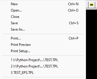
| Пункт | Перевод | Клавиша | Действие |
|---|---|---|---|
| New | Создать | Ctrl+N |
Новый пустой шаблон. |
| Open… | Открыть | Ctrl+O |
Открыть .tpl-файл. |
| Close | Закрыть | — | Закрыть текущий документ. |
| Save | Сохранить | Ctrl+S |
Сохранить документ. |
| Save As… | Сохранить как | — | Сохранить под другим именем. |
| Print… | Печать | Ctrl+P |
Печать изображения. |
| Print Preview | Предпросмотр печати | — | Предварительный просмотр перед печатью. |
| Print Setup… | Параметры печати | — | Выбор принтера и параметров страницы. |
| (список 1, 2, 3…) | Недавние файлы | — | Быстрое открытие недавно использованных .tpl. |
| Exit | Выход | — | Закрыть программу. |
5.2. Edit (Правка)
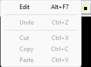
| Пункт | Перевод | Клавиша | Действие |
|---|---|---|---|
| Edit | Редактировать | Alt+F7 |
Открыть текущий .tpl во внешнем редакторе (задаётся в Config → Editor). |
| Undo | Отменить | Ctrl+Z |
Отмена (в текущем режиме недоступно — серый). |
| Cut / Copy / Paste | Вырезать / Копировать / Вставить | Ctrl+X / Ctrl+C / Ctrl+V |
Стандартные команды буфера обмена (недоступны — серые). |
5.3. View (Вид)
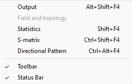
| Пункт | Перевод | Клавиша | Действие |
|---|---|---|---|
| Output | Выходной сигнал | Alt+Shift+F4 |
Показать выходной сигнал во временно́й области. |
| Field and topology | Поле и топология | — | Показать поле вместе с топологией. (В текущем состоянии пункт может быть серым, пока нет данных.) |
| Statistics | Статистика | Shift+F4 |
Открыть окно статистики расчёта (раздел 6). |
| S-matrix | S-матрица | Ctrl+Shift+F4 |
Показать S-матрицу рассеяния. |
| Directional Pattern | Диаграмма направленности | Ctrl+Alt+F4 |
Показать диаграмму направленности. |
| Toolbar | Панель инструментов | — | Показать/скрыть панель инструментов (галочка = показана). |
| Status Bar | Строка состояния | — | Показать/скрыть строку состояния (галочка = показана). |
5.4. Run (Расчёт)
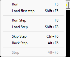
| Пункт | Перевод | Клавиша | Действие |
|---|---|---|---|
| Run | Запуск | F5 |
Расчёт от текущего такта до последнего. |
| Load first step | Загрузить первый шаг | Shift+F5 |
Вернуться к началу расчёта. |
| Run Step | Шаг расчёта | F8 |
Просчитать один текущий шаг. |
| Load Step | Загрузить шаг | Shift+F8 |
Перечитать текущий шаг. |
| Skip Step | Пропустить шаг | Ctrl+F6 |
Перейти на шаг вперёд без вывода. |
| Back Step | Шаг назад | Alt+F6 |
Вернуться на шаг назад. |
| Stop | Стоп | Alt+F5 |
Остановить идущий расчёт (активно только во время счёта). |
5.5. Config (Настройки)
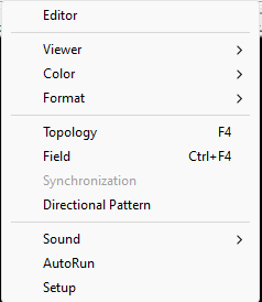
| Пункт | Перевод | Клавиша | Действие |
|---|---|---|---|
| Editor | Редактор | — | Указать путь к внешнему текстовому редактору для .tpl (раздел 6). |
| Viewer ► | Вьюверы | — | Подменю выбора внешних вьюверов (см. ниже). |
| Color ► | Цвет | — | Подменю настройки цвета. |
| Format ► | Формат | — | Подменю формата выходных файлов. |
| Topology | Топология | F4 |
Вывести топологию модели. |
| Field | Поле | Ctrl+F4 |
Вывести распределение поля. |
| Synchronization | Синхронизация | — | (Недоступно — серый.) |
| Directional Pattern | Диаграмма направленности | — | Настройка/вывод ДН. |
| Sound ► | Звук | — | Подменю звукового сопровождения. |
| AutoRun | Автозапуск | — | Автоматический запуск расчёта. |
| Setup | Настройка | — | Общие настройки. |
Подменю Config → Viewer — выбор внешних программ-вьюверов для просмотра каждого вида данных:
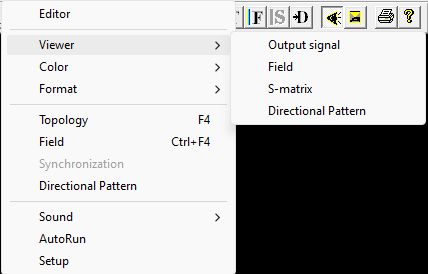
- Output signal — вьювер выходного сигнала (TMCROS);
- Field — вьювер поля (FieldView);
- S-matrix — вьювер S-матрицы (TMCGROUT);
- Directional Pattern — вьювер диаграммы направленности (TMC_DN).
Подменю Config → Color — настройка цвета:
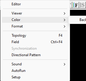
- BackGround — цвет фона рабочей области.
Подменю Config → Format — формат выходных файлов:
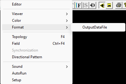
- OutputDataFile — настройка формата (точности печати чисел) выходного файла данных.
Подменю Config → Sound — звуковое сопровождение:
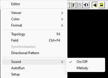
- On/Off — включить/выключить звук (галочка = включён);
- Melody — выбор мелодии.
5.6. Window (Окно)
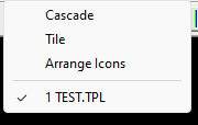
| Пункт | Перевод | Действие |
|---|---|---|
| Cascade | Каскадом | Расположить окна документов каскадом. |
| Tile | Мозаикой | Расположить окна мозаикой. |
| Arrange Icons | Упорядочить значки | Упорядочить свёрнутые окна. |
| (список 1 …) | Открытые документы | Переключение между открытыми .tpl (галочка — активный). |
5.7. Help (Справка)

| Пункт | Перевод | Действие |
|---|---|---|
| About PlanRT_H… | О программе | Сведения о версии программы. |
6. Диалоговые окна
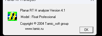
6.1. About (О программе)
Вызывается через Help → About PlanRT_H… или кнопкой .
Показывает название, версию и сведения о разработчике.
6.2. Statistics (Статистика расчёта)
Вызывается через View → Statistics (Shift+F4) или кнопкой .
Окно показывает параметры расчётной сетки и текущего расчёта.
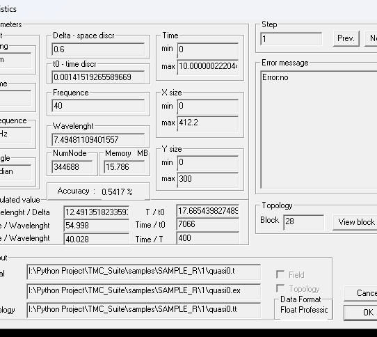
Основные поля:
- Parameters → Unit — единицы измерения:
Long(длина, напримерmm),Time(ns),Frequence(GHz),Angle(radian). - Delta - space discr — шаг пространственной дискретизации (Δ).
- t0 - time discr — шаг по времени.
- Frequence — рабочая частота.
- Wavelenght — длина волны.
- NumNode — число узлов сетки; Memory MB — объём занятой памяти.
- Time (min / max) — временно́й интервал расчёта.
- X size / Y size (min / max) — размеры расчётной области.
- Accuracy — оценка точности (в процентах).
- Calculated value — производные величины:
lenght / Delta,Xsize / Wavelenght,Ysize / Wavelenght,T / t0,Time / t0,Time / T. - Step — номер текущего шага, кнопки Prev. / Next для переключения шагов.
- Error message — сообщение об ошибке (
Error:no— ошибок нет). - Topology → Block — номер блока; View block list — список блоков.
- Output → Signal / Field / Topology — пути к выходным файлам; флажки Field / Topology; Data Format — формат данных (например,
Float Professional). - Кнопки OK (применить) и Cancel (отмена).
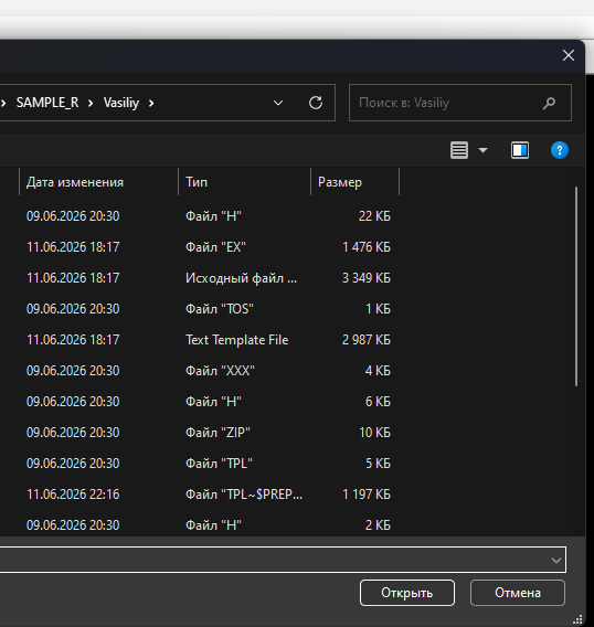
6.3. Выбор внешнего редактора (Config → Editor)
Команда Config → Editor открывает стандартное окно выбора файла, в котором нужно указать
исполняемый файл (.exe) внешнего текстового редактора. После этого команда Edit → Edit (Alt+F7)
будет открывать текущий .tpl именно в нём.
7. Входные данные: файл-шаблон .tpl
7.1. Что это и какое расширение
Главный входной файл программы — текстовый шаблон с расширением .tpl (text template). В нём
описаны: единицы измерения, параметры сетки и времени, топология (геометрия металла, поглотителей,
диэлектриков, входов), связи между блоками и какие выходные файлы создавать.
Как составить свой
.tplс нуля — методика (чертёж → «коробка» → декомпозиция на блоки → выбор шага сетки) и полный справочник входного языка со всеми ключевыми словами, рисунками примитивов и примерами:tpl-guide.md. Ниже — только краткий разбор рабочего примера.
Перед расчётом файл проходит препроцессинг библиотекой PREPR (раскрываются #include и #define,
вычисляются выражения). То есть .tpl можно писать «по-программистски»: с подключаемыми файлами и
именованными константами.
7.2. Сопутствующие файлы
Часто .tpl сам по себе короткий и лишь подключает заголовочные файлы .h:
.tpl— главный файл (точка входа), задаёт сигнатуру, подключения и вызов макроса расчёта;.h— подключаемые файлы с константами (#define) и большими блоками топологии (макросы);.eps— файл распределения диэлектрической проницаемости ε (если используется неоднородная среда).
7.3. Разбор примера
Рассмотрим рабочий пример samples/SAMPLE_R/1/TEST.TPL:
#TMC_RT_H
#include horns.h
#include cir_quas.h

Wozmush    3.141592653589/8; quasi0; 40.0;

#EOF
Построчно:
| Строка | Значение |
|---|---|
#TMC_RT_H |
Сигнатура файла — обязательная первая строка, говорит ядру H, что это его шаблон. |
#include horns.h |
Подключить файл с константами геометрии (см. ниже). |
#include cir_quas.h |
Подключить файл, где определён макрос Wozmush — он разворачивается в полное описание расчётного шага (#STEP). |
Wozmush 3.141592653589/8; quasi0; 40.0; |
Вызов макроса с тремя параметрами: сдвиг sdvig = π/8, имя выходного файла quasi0, частота 40.0 ГГц. |
#EOF |
Признак конца файла. |
Комментарии и спецсимволы: - строки, начинающиеся с
#— директивы препроцессора (#include,#define,#STEP,#EOFи т. п.); - строки, начинающиеся с!— комментарии (поясняющий текст, игнорируется при разборе); -\\в конце строки — перенос (склейка) длинной строки макроса; -@ ( … )и@\\— служебные обёртки выражений препроцессора PREPR; - точка с запятой;разделяет параметры внутри команд.
7.4. Файл констант (horns.h)
Содержит только именованные константы — их удобно менять, не трогая геометрию:
#define L_box   @ ( 412.00)      // длина расчётной области по X
#define W_box   @ ( 300.00)      // ширина расчётной области по Y
#define W_input @ (   8.00)      // ширина входа
#define W_delta @ (   0.6)       // шаг сетки Δ
#define a2      @ ( 20 )         // геометрические размеры рупора …
#define apert   @ ( 39 )         // апертура
#define alfa    @ ( 7.36/180*3.141593 )   // угол (в радианах)
...
Каждый #define Имя @ ( Выражение ) задаёт константу. В выражениях можно использовать арифметику и
ранее объявленные константы (например, a1 определён через W_input, h — через apert, W_input, th).
7.5. Файл шага расчёта (cir_quas.h)
Здесь определён макрос Wozmush, который разворачивается в полный блок #STEP … #END_STEP. Внутри —
четыре секции:
Секция #PARM … #END_PARM — параметры расчёта:
| Параметр | Назначение |
|---|---|
ANGLE_UNIT radian; |
Единица углов (радианы). |
FREQ_UNIT GHz; |
Единица частоты (ГГц). |
LONG_UNIT mm; |
Единица длины (мм). |
TIME_UNIT ns; |
Единица времени (нс). |
DELTA W_delta; |
Пространственный шаг сетки Δ. |
TIME 0.; 10.; |
Временно́й интервал расчёта (от 0 до 10). |
X_MIN / X_MAX |
Границы области по X (0 … L_box). |
Y_MIN / Y_MAX |
Границы области по Y (0 … W_box). |
FREQ freq__; |
Рабочая частота (берётся из параметра макроса). |
Секция #TOPOLOGY … #END_TOPOLOGY — геометрия модели. Состоит из блоков:
 BLOCK 1;                         // номер блока
 POLYGON_STAT METAL;              // тип элемента и материал
   L   0;   a1/2;                 // вершины полигона (координаты L x; y;)
   L   a2;  a1/2;
   L   a2;  a1/2+W_delta;
 END_B                            // конец блока
Типы элементов топологии, встречающиеся в примере:
| Ключевое слово | Что задаёт |
|---|---|
POLYGON_STAT <материал> |
Полигон (ломаная), вершины задаются строками L x; y;. |
RECT_STAT <материал>; x1; x2; y1; y2; |
Прямоугольник по двум диапазонам координат. |
CIRCLE_STAT <выражение>; r1; r2; f1; f2; |
Кольцевой/круговой сегмент (диапазоны радиуса и угла). |
INPUT_X <тип>; y1; y2; t1; t2; |
Вход вдоль оси Y — ставится на левую или правую границу «коробки», размеры задаются по Y в диапазоне y1…y2, радиоимпульс во временно́м окне t1…t2. |
INPUT_Y <тип>; x1; x2; t1; t2; |
Вход вдоль оси X — ставится на нижнюю или верхнюю границу, размеры задаются по X. |
FILE <имя>; x1; x2; y1; y2; |
Загрузка распределения (например ε) из файла на прямоугольной области. |
Материалы: METAL (идеальный проводник), MAGNETIC (магнетик — стенка холостого хода),
ABSORBER (поглотитель). Вместо материала может стоять выражение (для неоднородной среды),
например в блоке 20: CIRCLE_STAT amp*cos(tpg*r0*(f-f0+sdvig__))/exp(...); — задаёт распределение
возмущения как функцию координат r, f (радиус, угол) и параметра sdvig__.
Выражение задаёт добавку ε⁺ к проницаемости вакуума, а не саму ε. Пластине с ε = 4 соответствует запись
3. Отсюда конструкция(W_eps-1), которая встречается во всех авторских заданиях.
INPUT_X— вход вдоль оси Y, а не «по оси X». Название означает ось, вдоль которой происходит возбуждение, а размеры входа задаются по перпендикулярной оси. Подробно — вtpl-guide.md, раздел 5.5.В строке 145 примера видна закомментированная альтернатива блока 28:
\\ FILE prof_rct ; …— символ\\в начале (после переноса) превращает строку в неиспользуемый вариант. Так в шаблонах хранят запасные варианты описания.
Секция #LINK_LIST … #END_LINK — связи блоков и плоскости симметрии:
 T 1; 0.0; W_box/2;     // блок 1 размещается в точке (x0=0.0, y0=W_box/2)
 ...
 T 20; R_vessel+l+a2; W_box/2;
Строка T <номер блока>; x0; y0; размещает блок с указанным номером в координатах (x0, y0)
(в единицах из секции #PARM). То есть в #TOPOLOGY блок описывается «в своей» системе координат, а в
#LINK_LIST ему назначается положение в общей расчётной области.
Секция #OUTPUT … #END_OUTPUT — какие выходные файлы создавать:
 FILE filename__;                              // базовое имя выходных файлов (= quasi0)
 FIELD_DISTRIBUTION_M filename__; freq__; 7; 8; // сохранить распределение поля на частоте freq, шаги 7 и 8
| Команда | Назначение |
|---|---|
FILE <имя>; |
Базовое имя для выходных файлов. Обязательна, должна быть первой; имя не должно содержать точку. |
SMATRIX <Sfile>; <частота>; <T_min>; <T_max>; |
Записать S-матрицу в Sfile.s для указанной частоты, усреднив по интервалу T_min…T_max. |
TOPOLOGY; |
Вывести топологию в <имя>.tt. |
FIELDS; |
Вывести распределение полей. Требует также TOPOLOGY;. Сильно замедляет счёт. |
FIELD_DISTRIBUTION <имя>; <частота>; <expr>; <expr>; |
Сохранить комплексное распределение поля (модуль → .em, фаза → .ef). |
FIELD_DISTRIBUTION_M <имя>; <частота>; <expr>; <expr>; |
То же, вариант с накоплением в памяти. |
Каждый
#STEPдаёт одну частотную точку в.s. Частотная характеристика получается свипом — многими шагами с разнымиFREQ, пишущими в один и тот жеSfile.
7.6. Как подготовить свои данные
- Скопируйте рабочий пример (
TEST.TPL+horns.h+cir_quas.h) в отдельную папку. - В
horns.hпоменяйте константы под свою задачу (размеры областиL_box/W_box, шагW_delta, геометрию рупора и т. д.). - При необходимости отредактируйте топологию в
cir_quas.h(блокиBLOCK … END_B). - В
.tplзадайте параметры запуска: сдвиг, имя выходного файла, частоту. - Откройте
.tplв программе и запустите расчёт (раздел 8).
Для правки удобно настроить внешний редактор (Config → Editor) и открывать файл прямо из программы
командой Edit → Edit (Alt+F7).
8. Выходные данные
После расчёта ядро создаёт файлы (имена строятся от базового имени, заданного в секции #OUTPUT):
| Расширение | Содержимое | Чем смотреть |
|---|---|---|
.t |
Временно́й сигнал на входах (падающие и отражённые волны) | TMCROS |
.s |
S-матрица рассеяния | TMCGROUT |
.tt |
Топология модели | FieldView |
.ex |
Распределение поля Ex (двоичный файл) | FieldView |
.ey |
Распределение поля Ey | FieldView |
.hz |
Распределение поля Hz | FieldView |
.em |
Модуль комплексного распределения поля | FieldView |
.ef |
Фаза комплексного распределения поля | FieldView |
.q, .ix, .iy |
Служебные файлы | — |
.eps |
Распределение диэлектрической проницаемости ε | ядро (вход и выход) |
Имена всех файлов строятся от базового имени, заданного строкой FILE в секции #OUTPUT. Список
проверен по коду (src/libs/TMCIndan/TmcRTH_IndanOutput.cpp, строки 194–204).
Расширение
.tfвстречается в авторском руководстве 2000 года и в списке форматов, которые открывает FieldView (*.tf;*.AMP;*.FAZ;*.ex). Текущий код его не пишет — это историческое расширение версии 2.0p.Файлы диаграммы направленности (
.dopдля TMC_DN) ядро напрямую не пишет — данные для ДН экспортируются отдельной подсистемой; см. API-документациюdocs/api/libs/tmcindan.md.
9. Типовые сценарии
Открыть готовый расчёт и посмотреть результат:
1. File → Open… → выбрать .tpl.
2. Config → Topology (F4) — убедиться, что топология отрисовалась правильно.
3. Run → Run (F5) — выполнить расчёт.
4. View → Output (Alt+Shift+F4) — посмотреть выходной сигнал; View → S-matrix — S-матрицу.
Пошаговый расчёт (для наблюдения за полем):
1. Run → Load first step (Shift+F5) — встать в начало.
2. Run → Run Step (F8) — просчитать один шаг; повторять.
3. Config → Field (Ctrl+F4) — наблюдать распределение поля на каждом шаге.
4. Run → Back Step / Skip Step — двигаться по тактам назад/вперёд.
Проверить параметры сетки и памяти перед длинным расчётом:
- View → Statistics (Shift+F4) — посмотреть число узлов, занятую память, шаги Δ и t0, оценку точности.
10. Возможные проблемы
| Симптом | Что проверить |
|---|---|
| Файл не открывается / ошибка разбора | Первая строка должна быть #TMC_RT_H; проверьте, что рядом лежат все #include-файлы (.h). |
| Рабочая область осталась чёрной | Выполните Config → Topology (F4) или запустите расчёт — пустой холст до вывода это нормально. |
Edit → Edit ничего не открывает |
Сначала укажите редактор в Config → Editor. |
В строке состояния Error ≠ no |
Откройте View → Statistics и посмотрите поле Error message. |
Кнопка Stop неактивна |
Она работает только во время идущего расчёта. |
| Долгий расчёт / нехватка памяти | Уменьшите область или увеличьте шаг DELTA; проверьте NumNode и Memory в окне статистики. |
11. Связанные программы и документы
- TMCROS — просмотр временно́го сигнала (
.t). См.tmcros.md. - TMCGROUT — просмотр S-матрицы (
.s). См.tmcgrout.md. - TMC_DN — просмотр диаграммы направленности. См.
tmc_dn.md. - FieldView — просмотр поля и топологии (
.ex,.tt). - PlanarRT_X — парное ядро для X-моды. См.
planar_rt_x.md. - API-документация ядра:
docs/api/kernels/planar_rt_h.md; формат данных:docs/api/libs/tmcindan.md.
User manual — the PlanarRT_H compute kernel (tmc_rth.exe)
Program: Planar RT H analyzer (the executable
tmc_rth.exe). The program's interface is in English — the manual gives the English item names as in the program, with a Russian/English explanation next to them. The captions on the screenshots are in Russian.
1. Purpose of the program
PlanarRT_H is a compute kernel of the TMC Suite package. It performs the electrodynamic computation of planar (two-dimensional) structures in H-polarization in the time domain: from a given topology (metal, absorbers, dielectrics, inputs) the program computes step by step how the electromagnetic field propagates and scatters.
In simple terms: you describe a "map" of the computation area in a text template
file .tpl, and the kernel "plays" a wave through it over time and saves the
results:
- the time signal at the inputs (
.t) — later viewed in the TMCROS viewer; - the scattering S-matrix (
.s) — viewed in the TMCGROUT viewer; - the field distribution (
.ex,.ey,.hz,.em,.ef) and the topology (.tt) — viewed in the FieldView viewer.
Thus PlanarRT_H is a "data generator": it computes, and separate viewer programs
draw the result. (The companion kernel PlanarRT_X does the same for the
X-mode — see planar_rt_x.md.)
2. Launching the program and opening data
- Launch the file
tmc_rth.exe(folderdist/win32/bin/). The main window opens (see the figure above). - Open a computation template file: menu File → Open… (or the
button on the toolbar, or
Ctrl+O). - In the file-selection dialog choose a file with the
.tplextension (for example,samples/SAMPLE_R/1/TEST.TPL). - After opening, the file name appears in the window title:
Planar RT H analyzer
   - [TEST.TPL]
.
You can also launch the program with a file at once, by dragging the
.tplonto the program icon or by giving the file path as a command-line argument:tmc_rth.exe "path\to\file.tpl".
3. The main window
The main window consists of five zones (shown with frames in the figure in section 1):
| Zone | Purpose |
|---|---|
| Title bar | The program name and the name of the open .tpl file. |
| Menu bar | All program commands: File, Edit, View, Run, Config, Window, Help. |
| Toolbar | Quick-access buttons for the most frequent commands. |
| Work area | Here the model topology, the field distribution and the graphs (signal / S-matrix / pattern) are drawn. Right after opening a file the area is black — the image appears after output or computation commands. |
| Status bar | On the left — Step (the number of the current computation step) and the Error indicator; in the center — Model (computation type/precision: Double for double precision, Float for single; in the current build — Double); on the right — Output (what is output, for example Signal). |
4. The toolbar
The toolbar duplicates the most useful menu items. The buttons from left to right are numbered:
| # | Button | Command (menu) | Shortcut | What it does |
|---|---|---|---|---|
| 1 | |
File → New | Ctrl+N |
Create a new (empty) template. |
| 2 | |
File → Open | Ctrl+O |
Open an existing .tpl file. |
| 3 | |
Edit → Edit | Alt+F7 |
Open the current .tpl in an external text editor for editing. |
| 4 | |
View → Output | Alt+Shift+F4 |
Show the output signal (the time-domain result). |
| 5 | |
View → Field and topology | — | Show the field distribution together with the topology. |
| 6 | |
View → S-matrix | Ctrl+Shift+F4 |
Show the scattering S-matrix. |
| 7 | |
View → Directional Pattern | Ctrl+Alt+F4 |
Show the radiation pattern. |
| 8 | |
View → Statistics | Shift+F4 |
Open the computation statistics window (see section 6). |
| 9 | |
Run → Load first step | Shift+F5 |
Load the first step (return to the start of the computation). |
| 10 | |
Run → Run | F5 |
Run the computation from the current step to the last. |
| 11 | |
Run → Stop | Alt+F5 |
Stop a running computation. (Active only during a computation.) |
| 12 | |
Run → Run Step | F8 |
Compute one current step. |
| 13 | |
Run → Load Step | Shift+F8 |
Load (re-read) the current step. |
| 14 | |
Run → Skip Step | Ctrl+F6 |
Skip one step forward without output. |
| 15 | |
Run → Back Step | Alt+F6 |
Go one step back. |
| 16 | |
Config → Topology | F4 |
Output (draw) the model topology. |
| 17 | |
Config → Field | Ctrl+F4 |
Output (draw) the field. |
| 18 | |
Config → Synchronization | — | Synchronization. In the current version this item is unavailable (the icon is gray). |
| 19 | |
Config → Directional Pattern | — | Configure/output the radiation pattern. |
| 20 | |
Config → Sound | — | Sound accompaniment (on/off, melody). |
| 21 | |
Config → AutoRun | — | Automatic start of the computation. |
| 22 | |
File → Print | Ctrl+P |
Print the current image. |
| 23 | |
Help → About | — | About the program (version). |
Tip: hovering the cursor over a button in the program itself shows its English name as a tooltip, and a short description appears in the status bar.
5. The menus
5.1. File
| Item | Translation | Shortcut | Action |
|---|---|---|---|
| New | Create | Ctrl+N |
A new empty template. |
| Open… | Open | Ctrl+O |
Open a .tpl file. |
| Close | Close | — | Close the current document. |
| Save | Save | Ctrl+S |
Save the document. |
| Save As… | Save as | — | Save under a different name. |
| Print… | Ctrl+P |
Print the image. | |
| Print Preview | Print preview | — | Preview before printing. |
| Print Setup… | Print settings | — | Choose the printer and page parameters. |
| (list 1, 2, 3…) | Recent files | — | Quick opening of recently used .tpl files. |
| Exit | Exit | — | Close the program. |
5.2. Edit
| Item | Translation | Shortcut | Action |
|---|---|---|---|
| Edit | Edit | Alt+F7 |
Open the current .tpl in the external editor (set in Config → Editor). |
| Undo | Undo | Ctrl+Z |
Undo (unavailable in the current mode — gray). |
| Cut / Copy / Paste | Cut / Copy / Paste | Ctrl+X / Ctrl+C / Ctrl+V |
Standard clipboard commands (unavailable — gray). |
5.3. View
| Item | Translation | Shortcut | Action |
|---|---|---|---|
| Output | Output signal | Alt+Shift+F4 |
Show the output signal in the time domain. |
| Field and topology | Field and topology | — | Show the field together with the topology. (In the current state the item may be gray while there is no data.) |
| Statistics | Statistics | Shift+F4 |
Open the computation statistics window (section 6). |
| S-matrix | S-matrix | Ctrl+Shift+F4 |
Show the scattering S-matrix. |
| Directional Pattern | Radiation pattern | Ctrl+Alt+F4 |
Show the radiation pattern. |
| Toolbar | Toolbar | — | Show/hide the toolbar (a check mark = shown). |
| Status Bar | Status bar | — | Show/hide the status bar (a check mark = shown). |
5.4. Run
| Item | Translation | Shortcut | Action |
|---|---|---|---|
| Run | Run | F5 |
Compute from the current step to the last. |
| Load first step | Load first step | Shift+F5 |
Return to the start of the computation. |
| Run Step | Computation step | F8 |
Compute one current step. |
| Load Step | Load step | Shift+F8 |
Re-read the current step. |
| Skip Step | Skip step | Ctrl+F6 |
Move one step forward without output. |
| Back Step | Back step | Alt+F6 |
Go one step back. |
| Stop | Stop | Alt+F5 |
Stop a running computation (active only during a computation). |
5.5. Config
| Item | Translation | Shortcut | Action |
|---|---|---|---|
| Editor | Editor | — | Set the path to the external text editor for .tpl (section 6). |
| Viewer ► | Viewers | — | Submenu for choosing external viewers (see below). |
| Color ► | Color | — | Color settings submenu. |
| Format ► | Format | — | Submenu for the output-file format. |
| Topology | Topology | F4 |
Output the model topology. |
| Field | Field | Ctrl+F4 |
Output the field distribution. |
| Synchronization | Synchronization | — | (Unavailable — gray.) |
| Directional Pattern | Radiation pattern | — | Configure/output the pattern. |
| Sound ► | Sound | — | Sound accompaniment submenu. |
| AutoRun | AutoRun | — | Automatic start of the computation. |
| Setup | Setup | — | General settings. |
The Config → Viewer submenu — choosing external viewer programs for each kind of data:
- Output signal — the output-signal viewer (TMCROS);
- Field — the field viewer (FieldView);
- S-matrix — the S-matrix viewer (TMCGROUT);
- Directional Pattern — the radiation-pattern viewer (TMC_DN).
The Config → Color submenu — color settings:
- BackGround — the background color of the work area.
The Config → Format submenu — the output-file format:
- OutputDataFile — configure the format (number-printing precision) of the output data file.
The Config → Sound submenu — sound accompaniment:
- On/Off — turn the sound on/off (a check mark = on);
- Melody — choose the melody.
5.6. Window
| Item | Translation | Action |
|---|---|---|
| Cascade | Cascade | Arrange the document windows in a cascade. |
| Tile | Tile | Arrange the windows tiled. |
| Arrange Icons | Arrange icons | Arrange the minimized windows. |
| (list 1 …) | Open documents | Switch between the open .tpl files (a check mark — the active one). |
5.7. Help
| Item | Translation | Action |
|---|---|---|
| About PlanRT_H… | About | Information about the program version. |
6. Dialog windows
6.1. About
Invoked via Help → About PlanRT_H… or the
button. Shows the name, version
and developer information.
6.2. Statistics
Invoked via View → Statistics (Shift+F4) or the
button. The window shows the
parameters of the computation grid and the current computation.
Main fields:
- Parameters → Unit — units of measurement:
Long(length, e.g.mm),Time(ns),Frequence(GHz),Angle(radian). - Delta - space discr — the spatial discretization step (Δ).
- t0 - time discr — the time step.
- Frequence — the operating frequency.
- Wavelenght — the wavelength.
- NumNode — the number of grid nodes; Memory MB — the amount of memory used.
- Time (min / max) — the time interval of the computation.
- X size / Y size (min / max) — the dimensions of the computation area.
- Accuracy — an accuracy estimate (as a percentage).
- Calculated value — derived quantities:
lenght / Delta,Xsize / Wavelenght,Ysize / Wavelenght,T / t0,Time / t0,Time / T. - Step — the current step number, the Prev. / Next buttons for switching steps.
- Error message — an error message (
Error:no— no errors). - Topology → Block — the block number; View block list — the list of blocks.
- Output → Signal / Field / Topology — the paths to the output files; the
Field / Topology checkboxes; Data Format — the data format (for example,
Float Professional). - The OK (apply) and Cancel (cancel) buttons.
6.3. Choosing the external editor (Config → Editor)
The Config → Editor command opens the standard file-selection window in which
you specify the executable (.exe) of the external text editor. After that the
Edit → Edit (Alt+F7) command will open the current .tpl in it.
7. Input data: the .tpl template file
7.1. What it is and its extension
The program's main input file is a text template with the .tpl extension
(text template). It describes: the units of measurement, the grid and time
parameters, the topology (the geometry of the metal, absorbers, dielectrics,
inputs), the links between blocks, and which output files to create.
How to write your own
.tplfrom scratch — the methodology (drawing → the "box" → decomposition into blocks → choosing the grid step) and the complete reference of the input language with every keyword, figures of the primitives and examples:tpl-guide.md. Below is only a short walkthrough of a working example.
Before the computation the file goes through preprocessing by the PREPR
library (#include and #define are expanded, expressions are evaluated). That
is, a .tpl can be written "programmatically": with included files and named
constants.
7.2. Accompanying files
Often the .tpl itself is short and only includes header files .h:
.tpl— the main file (the entry point); it sets the signature, the includes, and the call of the computation macro;.h— included files with constants (#define) and large blocks of topology (macros);.eps— a file with the distribution of the permittivity ε (if an inhomogeneous medium is used).
7.3. Walkthrough of an example
Consider the working example samples/SAMPLE_R/1/TEST.TPL:
#TMC_RT_H
#include horns.h
#include cir_quas.h

Wozmush    3.141592653589/8; quasi0; 40.0;

#EOF
Line by line:
| Line | Meaning |
|---|---|
#TMC_RT_H |
The file signature — the mandatory first line; it tells the H kernel that this is its template. |
#include horns.h |
Include the file with the geometry constants (see below). |
#include cir_quas.h |
Include the file where the Wozmush macro is defined — it expands into the full description of the computation step (#STEP). |
Wozmush 3.141592653589/8; quasi0; 40.0; |
A macro call with three parameters: the shift sdvig = π/8, the output file name quasi0, the frequency 40.0 GHz. |
#EOF |
The end-of-file marker. |
Comments and special characters: - lines starting with
#are preprocessor directives (#include,#define,#STEP,#EOF, etc.); - lines starting with!are comments (explanatory text, ignored during parsing); -\\at the end of a line is a continuation (joining) of a long macro line; -@ ( … )and@\\are service wrappers of PREPR preprocessor expressions; - a semicolon;separates parameters within commands.
7.4. The constants file (horns.h)
Contains only named constants — they are convenient to change without touching the geometry:
#define L_box   @ ( 412.00)      // length of the computation area along X
#define W_box   @ ( 300.00)      // width of the computation area along Y
#define W_input @ (   8.00)      // input width
#define W_delta @ (   0.6)       // grid step Δ
#define a2      @ ( 20 )         // horn geometric dimensions …
#define apert   @ ( 39 )         // aperture
#define alfa    @ ( 7.36/180*3.141593 )   // angle (in radians)
...
Each #define Name @ ( Expression ) sets a constant. Expressions may use
arithmetic and previously declared constants (for example, a1 is defined through
W_input, h through apert, W_input, th).
7.5. The computation-step file (cir_quas.h)
Here the Wozmush macro is defined, which expands into the full block **`#STEP …
END_STEP`**. Inside there are four sections:
The #PARM … #END_PARM section — computation parameters:
| Parameter | Purpose |
|---|---|
ANGLE_UNIT radian; |
The angle unit (radians). |
FREQ_UNIT GHz; |
The frequency unit (GHz). |
LONG_UNIT mm; |
The length unit (mm). |
TIME_UNIT ns; |
The time unit (ns). |
DELTA W_delta; |
The spatial grid step Δ. |
TIME 0.; 10.; |
The time interval of the computation (from 0 to 10). |
X_MIN / X_MAX |
The X boundaries of the area (0 … L_box). |
Y_MIN / Y_MAX |
The Y boundaries of the area (0 … W_box). |
FREQ freq__; |
The operating frequency (taken from the macro parameter). |
The #TOPOLOGY … #END_TOPOLOGY section — the model geometry. It consists of
blocks:
 BLOCK 1;                         // block number
 POLYGON_STAT METAL;              // element type and material
   L   0;   a1/2;                 // polygon vertices (coordinates L x; y;)
   L   a2;  a1/2;
   L   a2;  a1/2+W_delta;
 END_B                            // end of the block
The topology element types that appear in the example:
| Keyword | What it sets |
|---|---|
POLYGON_STAT <material> |
A polygon (polyline); the vertices are given by L x; y; lines. |
RECT_STAT <material>; x1; x2; y1; y2; |
A rectangle by two coordinate ranges. |
CIRCLE_STAT <expression>; r1; r2; f1; f2; |
An annular/circular segment (ranges of radius and angle). |
INPUT_X <type>; y1; y2; t1; t2; |
An input along the Y axis — placed on the left or right boundary of the "box"; its extent is given along Y in the range y1…y2, with a radio pulse in the time window t1…t2. |
INPUT_Y <type>; x1; x2; t1; t2; |
An input along the X axis — placed on the bottom or top boundary; its extent is given along X. |
FILE <name>; x1; x2; y1; y2; |
Load a distribution (for example ε) from a file over a rectangular area. |
Materials: METAL (a perfect conductor), MAGNETIC (a magnetic — an
open-circuit wall), ABSORBER (an absorber).
Instead of a material an expression may be given (for an inhomogeneous
medium), for example in block 20:
CIRCLE_STAT amp*cos(tpg*r0*(f-f0+sdvig__))/exp(...); — it sets the perturbation
distribution as a function of the coordinates r, f (radius, angle) and the
parameter sdvig__.
An expression sets the addition ε⁺ to the permittivity of vacuum, not ε itself. A plate with ε = 4 corresponds to writing
3. Hence the construct(W_eps-1)found throughout the author's task files.
INPUT_Xis an input along the Y axis, not "along the X axis". The name refers to the axis along which the excitation travels, while the extent of the input is given along the perpendicular axis. Seetpl-guide.md, section 5.5, for details.
The #LINK_LIST … #END_LINK section — the block links and the symmetry plane:
 T 1; 0.0; W_box/2;     // block 1 is placed at the point (x0=0.0, y0=W_box/2)
 ...
 T 20; R_vessel+l+a2; W_box/2;
The line T <block number>; x0; y0; places the block with the given number at
the coordinates (x0, y0) (in the units from the #PARM section). That is, in
#TOPOLOGY a block is described "in its own" coordinate system, and in
#LINK_LIST it is assigned a position in the common computation area.
The #OUTPUT … #END_OUTPUT section — which output files to create:
 FILE filename__;                              // base name of the output files (= quasi0)
 FIELD_DISTRIBUTION_M filename__; freq__; 7; 8; // save the field distribution at the freq frequency, steps 7 and 8
| Command | Purpose |
|---|---|
FILE <name>; |
The base name for the signal/S-matrix output files. |
FIELD_DISTRIBUTION_M <name>; <frequency>; <step1>; <step2>; |
Save the field distribution (magnitude) at the given frequency for the given steps. |
7.6. How to prepare your own data
- Copy the working example (
TEST.TPL+horns.h+cir_quas.h) into a separate folder. - In
horns.hchange the constants for your task (the area dimensionsL_box/W_box, the stepW_delta, the horn geometry, etc.). - If needed, edit the topology in
cir_quas.h(theBLOCK … END_Bblocks). - In the
.tplset the launch parameters: the shift, the output file name, the frequency. - Open the
.tplin the program and run the computation (section 8).
For editing it is convenient to configure the external editor (Config → Editor)
and open the file directly from the program with the Edit → Edit (Alt+F7)
command.
8. Output data
After the computation the kernel creates files (the names are built from the base
name given in the #OUTPUT section):
| Extension | Contents | What to view it with |
|---|---|---|
.t |
The time signal at the inputs (incident and reflected waves) | TMCROS |
.s |
The scattering S-matrix | TMCGROUT |
.tt |
The model topology | FieldView |
.ex |
The Ex field distribution (a binary file) | FieldView |
.ey |
The Ey field distribution | FieldView |
.hz |
The Hz field distribution | FieldView |
.em |
The magnitude of the complex field distribution | FieldView |
.ef |
The phase of the complex field distribution | FieldView |
.q, .ix, .iy |
Service files | — |
.eps |
The distribution of the permittivity ε | the kernel (input and output) |
All file names are built from the base name given by the FILE line in the
#OUTPUT section. The list has been verified against the code
(src/libs/TMCIndan/TmcRTH_IndanOutput.cpp, lines 194–204).
The extension
.tfappears in the author's 2000 manual and in the list of formats FieldView opens (*.tf;*.AMP;*.FAZ;*.ex). The current code does not write it — it is a historical extension of version 2.0p.The kernel does not write the radiation-pattern files (
.dopfor TMC_DN) directly — the data for the pattern is exported by a separate subsystem; see the API documentationdocs/api/libs/tmcindan.md.
9. Typical scenarios
Open a ready computation and view the result:
1. File → Open… → select a .tpl.
2. Config → Topology (F4) — make sure the topology is drawn correctly.
3. Run → Run (F5) — perform the computation.
4. View → Output (Alt+Shift+F4) — view the output signal; View → S-matrix —
the S-matrix.
Step-by-step computation (to observe the field):
1. Run → Load first step (Shift+F5) — go to the start.
2. Run → Run Step (F8) — compute one step; repeat.
3. Config → Field (Ctrl+F4) — observe the field distribution at each step.
4. Run → Back Step / Skip Step — move back/forward through the steps.
Check the grid and memory parameters before a long computation:
- View → Statistics (Shift+F4) — view the number of nodes, the memory used, the
Δ and t0 steps, and the accuracy estimate.
10. Possible problems
| Symptom | What to check |
|---|---|
| The file does not open / a parsing error | The first line must be #TMC_RT_H; check that all #include files (.h) are next to it. |
| The work area stayed black | Run Config → Topology (F4) or start the computation — an empty canvas before output is normal. |
Edit → Edit opens nothing |
First specify the editor in Config → Editor. |
In the status bar Error ≠ no |
Open View → Statistics and look at the Error message field. |
The Stop button is inactive |
It works only during a running computation. |
| A long computation / not enough memory | Reduce the area or increase the DELTA step; check NumNode and Memory in the statistics window. |
11. Related programs and documents
- TMCROS — viewing the time signal (
.t). Seetmcros.md. - TMCGROUT — viewing the S-matrix (
.s). Seetmcgrout.md. - TMC_DN — viewing the radiation pattern. See
tmc_dn.md. - FieldView — viewing the field and topology (
.ex,.tt). - PlanarRT_X — the companion kernel for the X-mode. See
planar_rt_x.md. - The kernel API documentation:
docs/api/kernels/planar_rt_h.md; the data format:docs/api/libs/tmcindan.md.