Руководство пользователя — программа TMCROS (TMCROS.exe)
Пакет TMC Suite. Это руководство написано простым языком и рассчитано на пользователя, который видит программу впервые. Все названия пунктов меню и кнопок приведены так, как они выглядят в программе (интерфейс — английский), а рядом дан перевод и пояснение.
1. Назначение программы
TMCROS (полное название в заголовке окна — Tamic Rt Output Signal Viewer, «просмотрщик выходного сигнала Tamic Rt») — это программа для просмотра временны́х сигналов. Проще говоря, она строит графики, у которых:
- по горизонтальной оси (X) отложено время — в отсчётах (номерах точек) либо в секундах и их долях (мс, мкс, нс, пс);
- по вертикальной оси (Y) отложен сигнал во времени либо вычисленная по нему величина — амплитудная огибающая, фаза (в радианах или градусах), КСВН или потери в децибелах.
Откуда берутся эти сигналы? Их рассчитывают счётные ядра пакета — tmc_rth (H-поляризация) и tmc_rtx (X-мода). При расчёте планарной структуры ядро может сохранить временно́й сигнал многополюсника — как меняется во времени отклик в каждом порту (входе). TMCROS читает этот сигнал из файла .t и показывает его в виде наглядного графика.
Что умеет программа:
- открывать готовые документы-графики (файлы
.tos) или напрямую файлы временно́го сигнала (.t); - показывать сразу несколько кривых на одном поле (например, сигналы с разных входов или из разных файлов);
- менять масштаб (увеличение/уменьшение, автоподбор по осям), сдвигать видимую область;
- настраивать цвета фона, сетки, осей и самих кривых, а также шрифт подписей;
- печатать график и сохранять настройки оформления в самом документе
.tos; - главная особенность — преобразовывать временно́й сигнал обратно в матрицу рассеяния (S-матрицу) на заданных частотах. Эта функция называется To S-matrix (подсистема «время → S-матрица», TtoS) и описана в разделе 6.7.
Чем TMCROS отличается от «соседней» программы TMCGROUT? TMCGROUT показывает частотные характеристики (S-матрицу в зависимости от частоты), а TMCROS показывает временны́е сигналы. Внешне они очень похожи (сделаны по одной схеме), поэтому меню и кнопки у них почти одинаковые. Но TMCROS дополнительно умеет восстанавливать S-матрицу из сигнала — этого в TMCGROUT нет.
Обратите внимание: TMCROS только показывает и преобразует уже посчитанные данные. Сам расчёт сигнала выполняют счётные ядра (
tmc_rth,tmc_rtx). Как получить файл.t, описано в разделе 7.
2. Запуск и открытие данных
Как запустить программу
- Найдите файл
TMCROS.exe(после сборки он лежит в каталогеdist/win32/binилиdist/win64/bin). - Запустите его двойным щелчком.
- При первом запуске программа разворачивается на весь экран. Если ранее уже открывались какие-либо файлы, TMCROS попытается автоматически открыть последний из них (список «недавних файлов» хранится в реестре Windows в разделе
TMCROS).
Какой файл открывать
TMCROS работает с двумя типами файлов (подробно — в разделе 7):
| Файл | Что это | Когда открывать |
|---|---|---|
.tos |
Документ TMCROS: текстовый файл с настройками графиков и ссылкой на файл(ы) .t |
Обычный способ. Сохраняет цвета, масштаб, список кривых |
.t |
Файл временно́го сигнала (результат расчётного ядра) | Если хотите быстро посмотреть «сырой» результат. Программа сама создаст для него документ |
Чтобы открыть файл:
- Меню File → Open… (Файл → Открыть), либо нажмите кнопку «Открыть» на панели инструментов, либо клавиши Ctrl+O.
- В диалоге выберите нужный
.tosили.tфайл. - График сигнала появится в окне документа.
Если вы открываете
.t-файл, рядом с ним будет создан документ (он хранит настройки отображения). В дальнейшем удобнее открывать именно документ.
3. Главное окно
Главное окно — это многодокументное окно (MDI): внутри него могут быть открыты сразу несколько окон с разными графиками.
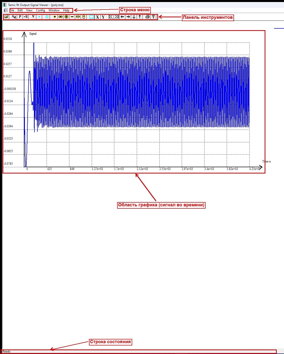
Окно состоит из четырёх зон:
- Строка меню (вверху) — все команды программы, сгруппированные по разделам (File, Edit, View, Config, Window, Help). Подробно — раздел 5.
- Панель инструментов (тулбар) — ряд кнопок-значков для самых частых действий. Подробно — раздел 4.
- Область графика (центр) — здесь рисуются оси, координатная сетка и сами кривые сигнала. По этой области работает мышь: можно выделить прямоугольник для увеличения (zoom), а двойной щелчок подгоняет масштаб.
- Строка состояния (статусбар) (внизу) — две панели: - левая — координаты точки под курсором мыши (значение времени по X и значение сигнала по Y); - правая — служебная информация о текущем графике (тип характеристики, отложенной по оси Y: сигнал, амплитуда, фаза, КСВН или потери).
4. Панель инструментов
Панель инструментов дублирует самые частые команды меню в виде кнопок. Если панель не видна, включите её через View → Toolbar.

Кнопки идут слева направо. Ниже — назначение каждой. Перечень и порядок взяты из ресурса программы (IDR_MAINFRAME TOOLBAR в файле src/viewers/Tmcrtout/TMCGROUT.rc), а пояснения — из таблицы подсказок (STRINGTABLE) того же файла. Тонкие вертикальные промежутки на панели — это разделители (SEPARATOR), они группируют кнопки по смыслу.
| № | Кнопка | Команда (ID) | Название (англ./рус.) | Что делает |
|---|---|---|---|---|
| 1 |  |
ID_FILE_OPEN |
Open / Открыть файл | Открывает файл .tos или .t (то же, что File → Open) |
| 2 |  |
ID_EDIT_ADDCHARACTERISTICS |
Add characteristics / Добавить характеристику | Добавляет в документ ещё одну кривую из выбранного .t-файла |
| 3 |  |
ID_EDIT_DOCUMENT |
Characteristics / Таблица графиков | Открывает таблицу со списком всех кривых документа (имена, файлы, входы/моды, флаги показа) |
| 4 |  |
ID_EDIT_TOSMATRIX |
To S-matrix / В S-матрицу | Открывает диалог преобразования сигнала в S-матрицу (главная функция TMCROS, раздел 6.7) |
| 5 |  |
ID_EDIT_GRAPHICSPARAMETERS |
Viewport / Параметры окна | Открывает диалог настройки отображения: пределы по осям, единицы времени, тип характеристики Y, формат подписей, точки |
| 6 |  |
ID_VIEW_GRAPHICS |
Redraw data / Перечитать и перерисовать | Заново читает данные из файлов и перерисовывает график |
| 7 |  |
ID_VIEW_RESIZECTRLR |
Resize viewport / Подогнать область графика | Подгоняет область рисования под размер окна |
| 8 |  |
ID_VIEW_ZOOM_ZOOMP |
Zoom + / Увеличить | Увеличивает масштаб по обеим осям |
| 9 |  |
ID_VIEW_ZOOM_ZOOMXP |
Zoom +X / Увеличить по X | Увеличивает масштаб только по горизонтали (времени) |
| 10 |  |
ID_VIEW_ZOOM_ZOOMYP |
Zoom +Y / Увеличить по Y | Увеличивает масштаб только по вертикали (сигналу) |
| 11 |  |
ID_VIEW_ZOOM_ZOOM |
Zoom − / Уменьшить | Уменьшает масштаб по обеим осям |
| 12 |  |
ID_VIEW_ZOOM_ZOOMX |
Zoom −X / Уменьшить по X | Уменьшает масштаб только по горизонтали |
| 13 |  |
ID_VIEW_ZOOM_ZOOMY |
Zoom −Y / Уменьшить по Y | Уменьшает масштаб только по вертикали |
| 14 |  |
ID_VIEW_RESIZEWINDOW |
Resize window / Подогнать окно данных | Подгоняет вещественные пределы (окно данных) |
| 15 |  |
ID_VIEW_AUTOXSIZE |
Auto X size / Авто-масштаб X | Автоматически подбирает пределы по оси X (времени) под данные |
| 16 |  |
ID_VIEW_AUTOYSIZE |
Auto Y size / Авто-масштаб Y | Автоматически подбирает пределы по оси Y под данные |
| 17 |  |
ID_VIEW_TRANSLATE_CHANGEXMAXXMIN_HOME |
Change Xmin auto (Home) / В начало | Переход к началу диапазона по X (клавиша Home) |
| 18 |  |
ID_VIEW_TRANSLATE_CHANGEXMAXXMIN_END |
Change Xmax auto (End) / В конец | Переход к концу диапазона по X (клавиша End) |
| 19 |  |
ID_VIEW_CHANGEXMAXXMIN_DECRIMENT |
Decrement Xmin/Xmax / Сдвиг влево | Сдвигает видимую область по времени влево |
| 20 |  |
ID_VIEW_CHANGEXMAXXMIN_INCREMENT |
Increment Xmin/Xmax / Сдвиг вправо | Сдвигает видимую область по времени вправо |
| 21 |  |
ID_VIEW_CHANGEYMAXYMIN_DECREMENT |
Decrement Ymin/Ymax / Сдвиг вниз | Сдвигает видимую область вниз |
| 22 |  |
ID_VIEW_CHANGEYMAXYMIN_INCREMENT |
Increment Ymin/Ymax / Сдвиг вверх | Сдвигает видимую область вверх |
| 23 |  |
ID_FILE_PRINT |
Print / Печать | Печатает текущий график (то же, что File → Print) |
| 24 |  |
ID_APP_ABOUT |
About / О программе | Показывает окно «О программе TMCROS» |
5. Меню
Ниже разобран каждый пункт каждого меню: что он делает, какая у него горячая клавиша и что происходит после выбора. Структура взята из ресурса меню IDR_TMCGROTYPE (меню при открытом документе).
5.1. Меню File (Файл)
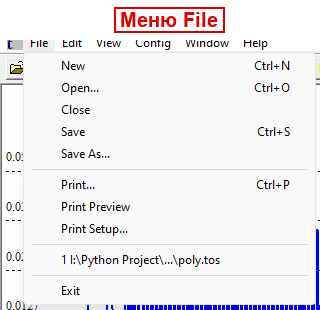
| Пункт | Горячая клавиша | Что делает |
|---|---|---|
| New (Создать) | Ctrl+N | Создаёт новый пустой документ-график |
| Open… (Открыть) | Ctrl+O | Открывает существующий .tos или .t файл |
| Close (Закрыть) | — | Закрывает текущее окно документа |
| Save (Сохранить) | Ctrl+S | Сохраняет текущий документ (.tos) вместе со всеми настройками оформления |
| Save As… (Сохранить как) | — | Сохраняет документ под новым именем |
| Print… (Печать) | Ctrl+P | Печатает график |
| Print Preview (Предпросмотр печати) | — | Показывает, как график будет выглядеть на бумаге |
| Print Setup… (Параметры печати) | — | Настройки принтера и страницы |
| Recent File / список последних файлов | — | Быстрое открытие недавно использованных документов |
| Exit (Выход) | — | Закрывает программу |
При сохранении настройки оформления (цвета, шрифт, типы линий) дополнительно запоминаются в реестре Windows и используются как значения по умолчанию для новых документов.
5.2. Меню Edit (Правка)
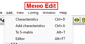
| Пункт | Горячая клавиша | Что делает |
|---|---|---|
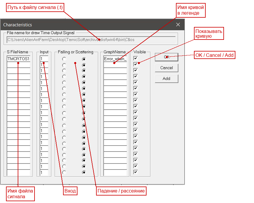
| Characteristics (Характеристики / таблица графиков) | Ctrl+D | Открывает таблицу содержимого документа: список всех кривых (до 20). Для каждой видно имя графика, имя .t-файла, входы/моды и флаг «показывать/не показывать» |
| Add characteristics (Добавить характеристику) | Ctrl+A | Открывает диалог выбора .t-файла и добавляет из него новую кривую в текущий документ |
| To S-matrix (В S-матрицу) | Alt+T | Открывает диалог преобразования временно́го сигнала в матрицу рассеяния (главная функция TMCROS). Подробно — раздел 6.7 |
| Editor (Внешний редактор) | Alt+F7 | Открывает файл документа во внешнем текстовом редакторе — для ручного редактирования .tos |
5.3. Меню View (Вид)
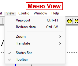
| Пункт | Горячая клавиша | Что делает |
|---|---|---|
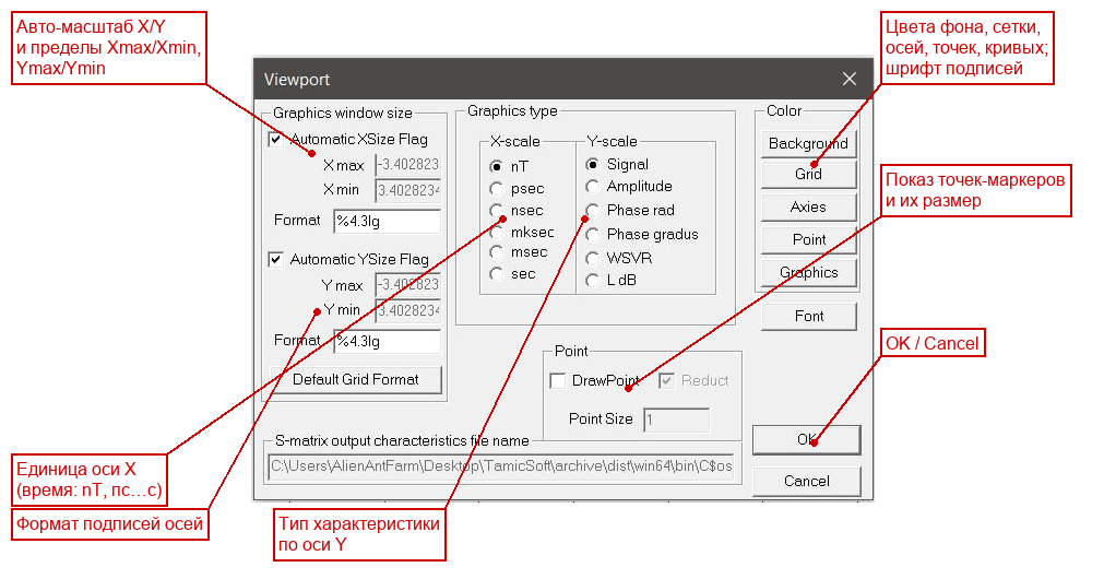
| Viewport (Параметры окна) | Ctrl+H | Открывает диалог настройки отображения: пределы Xmin/Xmax/Ymin/Ymax, авто-масштаб, единица оси X (время), тип характеристики Y, формат подписей, показ точек-маркеров |
| Redraw data (Перечитать и перерисовать) | Ctrl+W | Заново читает данные из файлов и перерисовывает график. Полезно, если файл .t пересчитан заново |
| Zoom ► (Масштаб) | — | Подменю масштабирования (см. ниже) |
| Translate ► (Сдвиг) | — | Подменю сдвига границ области (см. ниже) |
| Status Bar (Строка состояния) | — | Включает/выключает нижнюю строку состояния |
| Toolbar (Панель инструментов) | — | Включает/выключает панель инструментов |
Подменю View → Zoom (Масштаб)
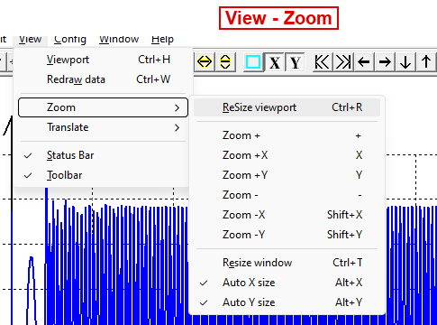
| Пункт | Горячая клавиша | Что делает |
|---|---|---|
| ReSize viewport (Подогнать область) | Ctrl+R | Подгоняет область рисования под текущее окно |
| Zoom + (Увеличить) | + | Увеличивает масштаб по обеим осям |
| Zoom +X (Увеличить по X) | X | Увеличивает масштаб только по времени |
| Zoom +Y (Увеличить по Y) | Y | Увеличивает масштаб только по вертикали |
| Zoom − (Уменьшить) | − | Уменьшает масштаб по обеим осям |
| Zoom −X (Уменьшить по X) | Shift+X | Уменьшает масштаб по времени |
| Zoom −Y (Уменьшить по Y) | Shift+Y | Уменьшает масштаб по вертикали |
| Resize window (Подогнать окно данных) | Ctrl+T | Изменяет вещественные пределы окна данных |
| Auto X size (Авто-масштаб X) | Alt+X | Включает автоматический подбор пределов по X. В меню появляется галочка |
| Auto Y size (Авто-масштаб Y) | Alt+Y | Включает автоматический подбор пределов по Y. В меню появляется галочка |
При включённом авто-масштабе по оси программа сама подбирает пределы под минимум/максимум данных, и ручные пределы по этой оси игнорируются (поля Xmin/Xmax или Ymin/Ymax в диалоге Viewport становятся недоступны).
Подменю View → Translate (Сдвиг)
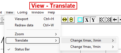
| Пункт | Вложенные команды | Что делает |
|---|---|---|
| Change Xmax, Xmin ► | Decrement (← / стрелка влево), Increment (→ / стрелка вправо), Home (Home), End (End) | Сдвиг видимой области по времени влево/вправо, а также переход к началу (Home) и концу (End) диапазона |
| Change Ymax, Ymin ► | Decrement (V / стрелка вниз), Increment (^ / стрелка вверх) | Сдвиг видимой области вверх/вниз |
Сдвиг удобен, когда нужно «прокрутить» график влево/вправо/вверх/вниз, не меняя масштаб. Шаг сдвига — порядка 10 % текущего диапазона.
5.4. Меню Config (Настройки)
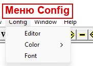
| Пункт | Что делает |
|---|---|
| Editor (Редактор) | Задаёт путь к внешнему текстовому редактору для .tos-файлов |
| Color ► (Цвет) | Подменю выбора цветов элементов графика (см. ниже) |
| Font (Шрифт) | Открывает стандартный диалог выбора шрифта, размера и цвета подписей осей и сетки |
Подменю Config → Color (Цвет)
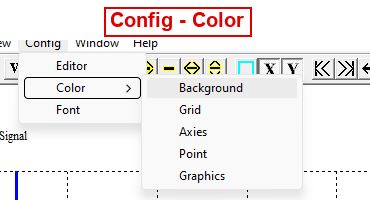
| Пункт | Что меняет |
|---|---|
| Background (Фон) | Цвет фона области графика |
| Grid (Сетка) | Цвет координатной сетки |
| Axies (Оси) | Цвет осей координат |
| Point (Точки) | Цвет точек-маркеров на кривых |
| Graphics (Графики) | Открывает диалог цветов/типов/толщины линий сразу для 16 кривых — здесь же можно задать индивидуальный цвет каждой кривой |
Пункт Graphics открывает таблицу из 16 образцов линий. Нажав на нужный образец, вы выбираете цвет, стиль (Solid — сплошная, Dash — пунктир, Dot — точки, DashDot, DashDotDot) и толщину этой линии.
5.5. Меню Window (Окно)
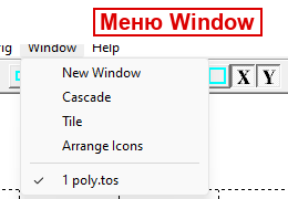
| Пункт | Что делает |
|---|---|
| New Window (Новое окно) | Открывает ещё одно окно для того же документа (полезно для разных масштабов одного графика) |
| Cascade (Каскад) | Располагает окна каскадом |
| Tile (Мозаика) | Располагает окна плиткой (рядом) |
| Arrange Icons (Упорядочить значки) | Выравнивает свёрнутые окна-значки |
| Список окон | Переключение между открытыми окнами документов |
5.6. Меню Help (Справка)
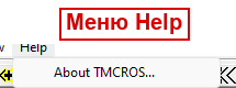
| Пункт | Что делает |
|---|---|
| About TMCROS… (О программе) | Показывает окно с названием и версией программы (Tamic Rt Output Signal Viewer) |
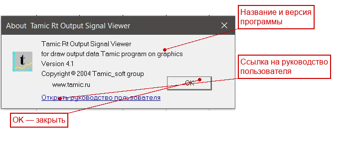
6. Типовые сценарии работы
Ниже — пошаговые инструкции для самых частых задач.
6.1. Открыть документ .tos
- Меню File → Open… (или Ctrl+O, или кнопка «Открыть» на панели).
- Выберите файл с расширением
.tos(например,poly.tos). - График сигнала построится автоматически. Если кривая «уехала» за пределы окна — нажмите кнопки авто-масштаба Auto X size и Auto Y size.
6.2. Открыть «сырой» сигнал .t
- Меню File → Open… (Ctrl+O).
- В диалоге выберите файл с расширением
.t(например,poly.t). - Программа прочитает сигнал и построит график; рядом будет создан документ для хранения настроек отображения. Сохраните его (File → Save, Ctrl+S), чтобы в следующий раз открывать уже готовый документ.
6.3. Добавить ещё одну характеристику (Add characteristics)
- Откройте документ (см. 6.1).
- Меню Edit → Add characteristics (Ctrl+A) или кнопка «Добавить характеристику».
- В диалоге выберите нужный
.t-файл. - Новая кривая добавится в документ. Чтобы посмотреть/настроить список всех кривых, откройте Edit → Characteristics (Ctrl+D).
- В таблице можно включать и выключать показ каждой кривой (флаг вывода), а также задавать вход/моду нужного столбца сигнала.
6.4. Настроить масштаб (Zoom / Auto X / Auto Y)
Есть три способа изменить масштаб:
- Мышью — зажмите левую кнопку и обведите прямоугольником интересующую область графика; при отпускании кнопки программа увеличит выделенное. Двойной щелчок в области графика подгоняет масштаб обратно.
- Кнопками панели — Zoom + / Zoom − (обе оси), Zoom +X/−X, Zoom +Y/−Y (по одной оси).
- Авто-масштаб — View → Zoom → Auto X size (Alt+X) и Auto Y size (Alt+Y). Программа сама подберёт пределы так, чтобы видеть всю кривую. Это самый быстрый способ «вписать» график в окно.
6.5. Сдвинуть график (Translate)
- Меню View → Translate.
- Выберите Change Xmax, Xmin (сдвиг по времени) или Change Ymax, Ymin (сдвиг по вертикали).
- Во вложенном подменю выберите Decrement или Increment (либо клавиши-стрелки). Для перехода в начало/конец диапазона по времени используйте Home/End.
Тот же эффект дают кнопки сдвига на панели инструментов (№17–22).
Сдвиг работает только при выключенном авто-масштабе по соответствующей оси: при включённом авто-масштабе пределы определяются автоматически по данным.
6.6. Сменить цвета и тип характеристики
Цвет фона / сетки / осей / точек: 1. Меню Config → Color → Background / Grid / Axies / Point. 2. В стандартном диалоге выберите цвет → OK.
Цвет, стиль и толщина кривых: 1. Меню Config → Color → Graphics. 2. В открывшейся таблице нажмите образец нужной кривой. 3. Выберите цвет, стиль линии (Solid/Dash/Dot/DashDot/DashDotDot) и толщину → OK.
Что отложено по оси Y и единицы оси X (время): 1. Меню View → Viewport (Ctrl+H) или кнопка «Параметры окна». 2. В диалоге выберите тип характеристики Y (Signal, Amplitude, WSVR, L dB, Phase rad, Phase grad) и единицу оси X (nT — отсчёты, либо pс/нс/мкс/мс/с), при желании задайте пределы и формат подписей → OK.
6.7. Восстановить S-матрицу из сигнала (To S-matrix)
Это главная, отличающая TMCROS функция. Она берёт один или несколько временны́х сигналов (.t) и вычисляет по ним матрицу рассеяния на заданных частотах, сохраняя результат в файл S-матрицы (.s). Полученный .s-файл затем можно открыть в программе TMCGROUT и смотреть как обычную частотную характеристику.
Идея метода (кратко). Временно́й сигнал на каждом входе считается гармоническим колебанием s(t) = A·sin(ω·t + φ) на заданной частоте. По соседним отсчётам сигнала программа восстанавливает амплитуду A и фазу φ — то есть комплексное значение элемента S-матрицы — и усредняет результат по выбранному диапазону времени. Вход, на котором есть сигнал (возбуждённый вход), определяет строку S-матрицы.
Пошагово:
- Откройте документ с сигналом (
.tos) или сам.t-файл. - Меню Edit → To S-matrix (Alt+T) или кнопка «В S-матрицу» на панели.
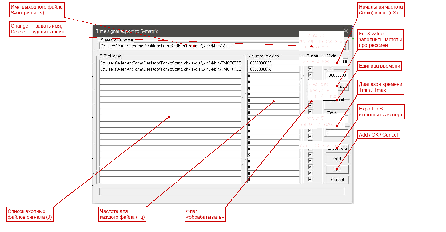
- Откроется диалог преобразования (см. рисунок ниже). В нём:
- список входных файлов
.t(до 20) с флажком «обрабатывать» у каждого. Кнопкой Add добавьте нужные файлы сигнала; - поле выходного
.s-файла — имя результата; по умолчанию это<имя документа>.s. Изменить его можно кнопкой Change, удалить файл с диска — кнопкой Delete; - частота для каждого входного файла (в Гц). Чтобы быстро заполнить столбец частот арифметической прогрессией (начальная частота + шаг), нажмите кнопку Fill X value;
- диапазон времени
Tmin/Tmaxи единица времени — задают, на каком участке сигнала выполняется восстановление. 4. Нажмите кнопку Export to S (или OK). Программа по очереди обработает все отмеченные файлы и запишет результат в один.s-файл. 5. Откройте полученный.sв TMCGROUT, чтобы увидеть восстановленную частотную характеристику.
6.8. Напечатать график
- Сначала настройте масштаб и оформление так, как хотите видеть на бумаге.
- (По желанию) Меню File → Print Preview — проверьте, как график ляжет на страницу.
- Меню File → Print… (Ctrl+P) или кнопка «Печать».
- Выберите принтер и нажмите OK.
7. Форматы входных данных
TMCROS работает с двумя форматами файлов: документ .tos и файл временно́го сигнала .t.
7.1. Файл документа .tos
.tos — это текстовый файл-документ TMCROS. Его можно открыть любым текстовым редактором. Он хранит настройки оформления и список кривых, но не хранит сами данные — данные берутся из файлов .t, на которые ссылается документ.
Структура файла (на примере реального файла samples/SAMPLE_R/ABSORBER/poly.tos):
#TMCGROTS
!Graphics parameters
!Graphics data
!file name : E:\BackUP\ARHIV\WORK\Source\SAMPLE_R\ABSORBER\poly.tos
!Data file for draw graphics
!TFileName GraphicsName DrawFlag Input1 Mod1 Input2 Mod2
poly.t poly.t 1 1 1 1 1
Разбор по строкам:
| Строка | Назначение |
|---|---|
#TMCGROTS |
Сигнатура — обязательная первая строка. По ней программа узнаёт «свой» файл документа |
Строки, начинающиеся с ! |
Комментарии — программа их игнорирует (включая авто-сгенерированный путь и подсказку по столбцам) |
Строки #Ключ значение |
Параметры оформления (в этом простом примере их нет, но они могут присутствовать — см. ниже) |
Последние строки (без #) |
Описания кривых — по одной строке на кривую |
Параметры оформления (#Ключ). В полном документе TMCROS могут присутствовать ключи настройки осей и цветов (по аналогии с документом TMCGROUT). Основные из них:
| Ключ | Что задаёт | Значения |
|---|---|---|
#nXType |
Тип оси X (единица времени) | 0 — отсчёты (nT), 1 — пс, 2 — нс, 3 — мкс, 4 — мс, 5 — с |
#nYType |
Тип оси Y (характеристика) | 0 — сигнал (Signal), 1 — амплитуда (Amplitude), 2 — фаза рад (Phase rad), 3 — фаза град (Phase grad), 4 — КСВН (WSVR), 5 — потери дБ (L dB) |
#Xmin, #Xmax |
Пределы по оси X (времени) | числа в выбранной единице |
#Ymin, #Ymax |
Пределы по оси Y | числа |
#nAFlagX / #nAFlagY |
Авто-масштаб по X / по Y | 0 — выкл, 1 — вкл |
#sDrawBckgrdColor / #sDrawGridColor / #sDrawAxiesColor / #sDrawPointColor / #sDrawTextColor |
Цвета фона, сетки, осей, точек, текста | числа COLORREF (16777215 = белый, 0 = чёрный) |
#sDrawTextFont |
Шрифт подписей | параметры шрифта (имя, размер и т.д.) |
#EditorFileName |
Внешний редактор документа | путь к .exe |
Описание кривой (строка данных). Формат столбцов указан в комментарии выше неё:
!TFileName GraphicsName DrawFlag Input1 Mod1 Input2 Mod2
poly.t     poly.t       1        1      1    1      1
| Столбец | Значение в примере | Назначение |
|---|---|---|
TFileName |
poly.t |
Имя файла временно́го сигнала (обычно относительный путь рядом с .tos) |
GraphicsName |
poly.t |
Подпись кривой в легенде |
DrawFlag |
1 |
Показывать кривую: 1 — да, 0 — нет |
Input1 |
1 |
Номер первого входа (порта) в файле сигнала |
Mod1 |
1 |
Номер моды/компоненты первого входа |
Input2 |
1 |
Номер второго входа |
Mod2 |
1 |
Номер моды/компоненты второго входа |
7.2. Файл временно́го сигнала .t
.t — это файл с самим временны́м сигналом многополюсника: для каждого момента времени хранятся отсчёты сигнала по всем входам (портам). Это результат работы счётного ядра (tmc_rth или tmc_rtx). Файл текстовый, его можно открыть любым редактором.
Начало файла (пример samples/SAMPLE_R/ABSORBER/poly.t):
#TMC_GraphicsOutputSignalFile FormVer2.0 2000
!File name E:\BackUP\ARHIV\WORK\Source\SAMPLE_R\ABSORBER\poly.t
#TMC_GROTS_Freq 1e+010
#TMC_GROTS_InpNum -2
!nT nBlock  Up  Uo
        0              0   7              0              0   8              0              0
        1  4.717309e-012   7      0.2920765    -0.05489582   8              0              0
        2  9.434617e-012   7      0.5586809     0.03530808   8              0              0
        ...
| Элемент | Что это |
|---|---|
#TMC_GraphicsOutputSignalFile FormVer2.0 2000 |
Сигнатура файла сигнала (версия формата 2.0, год 2000) |
!File name <путь> |
Комментарий с исходным путём к файлу (строки с ! игнорируются) |
#TMC_GROTS_Freq 1e+010 |
Частота (Гц), на которой считался сигнал — здесь 10 ГГц. Используется при восстановлении амплитуды/фазы и в функции To S-matrix |
#TMC_GROTS_InpNum -2 |
Служебная строка с числом входов |
!nT nBlock Up Uo |
Комментарий-подсказка с названиями столбцов |
| Строки данных (начинаются с пробела) | Сами отсчёты сигнала: для каждой точки — её номер, время и далее по каждому входу — номер входа и пара чисел (Re/Im отсчёта сигнала) |
Как читать строку данных (на примере точки №1):
1 4.717309e-012 7 0.2920765 -0.05489582 8 0 0
| Поле | Значение | Смысл |
|---|---|---|
1 |
номер точки | Порядковый номер отсчёта (он же «время в отсчётах», тип оси X = nT) |
4.717309e-012 |
время, с | Момент времени данного отсчёта (здесь ≈ 4.72 пс) |
7 0.2920765 -0.05489582 |
вход 7: Re, Im | Номер первого входа и пара значений сигнала (вещественная и мнимая часть отсчёта) |
8 0 0 |
вход 8: Re, Im | Номер второго входа и пара значений (здесь нули — вход не возбуждён) |
То есть в каждой строке после номера точки и времени идут тройки «номер входа + два числа» — по одной тройке на каждый вход (порт) структуры.
7.3. Как получить файлы .t и .tos
Файл .t создаётся счётным ядром при расчёте планарной структуры с выводом временно́го сигнала. Кратко (подробно — в docs/api/kernels/planar_rt_h.md и руководствах по ядрам):
- Подготовьте входной файл-шаблон
.tpl(топология структуры, параметры, секция вывода). В секции вывода должен быть включён вывод временно́го сигнала и задано имя выходного файла.t. - Запустите счётное ядро:
tmc_rth.exe(для H-поляризации) илиtmc_rtx.exe(для X-моды), откройте в нём.tplи выполните расчёт. - По завершении ядро запишет файл
.tс временны́м сигналом. - Откройте полученный
.tв TMCROS — программа автоматически создаст рядом документ. Дальше настройте оформление и сохраните (Ctrl+S).
Готовые примеры для тренировки лежат в samples/SAMPLE_R/ (например, ABSORBER/poly.t + poly.tos, а также 1/quasi0.tos).
8. Возможные проблемы и их решение
| Симптом | Причина | Что делать |
|---|---|---|
В легенде/области графика надпись Error_when_read… |
Файл .t не найден, пуст или повреждён |
Проверьте, существует ли .t-файл по указанному в .tos пути; пересчитайте его ядром заново |
| График пустой или кривая не видна | Включён неудачный масштаб, либо данные вне окна | Нажмите Auto X size и Auto Y size (Alt+X, Alt+Y), чтобы вписать кривую в окно |
| Кривая есть, но «уезжает» за край | Заданы ручные пределы Xmin/Xmax/Ymin/Ymax | Откройте View → Viewport и проверьте пределы, либо включите авто-масштаб |
После пересчёта .t график не обновился |
TMCROS показывает старые данные | Нажмите View → Redraw data (Ctrl+W) или кнопку «Перечитать» |
| Кривая одного цвета с фоном/её плохо видно | Совпали цвета | Config → Color → Graphics — задайте контрастный цвет линии |
| Функция To S-matrix выдаёт ошибку | Не выбран ни один файл, файл .t недоступен, мало точек в диапазоне Tmin..Tmax, не задана частота |
Проверьте список файлов и флажки, задайте корректный диапазон времени и частоты; убедитесь, что файл сигнала существует |
| Не открывается файл — сообщение про «не тот формат» | Первая строка документа не #TMCGROTS |
Убедитесь, что открываете корректный документ; первая строка .tos должна быть #TMCGROTS, а файла сигнала — #TMC_GraphicsOutputSignalFile… |
User manual — the TMCROS program (TMCROS.exe)
TMC Suite package. This manual is written in plain language and is intended for a user seeing the program for the first time. All menu and button names are given as they appear in the program (the interface is in English), with a translation and explanation next to them.
1. Purpose of the program
TMCROS (the full name in the window title is Tamic Rt Output Signal Viewer) is a program for viewing time signals. In simple terms, it builds graphs where:
- the horizontal axis (X) shows time — in samples (point numbers) or in seconds and fractions of them (ms, µs, ns, ps);
- the vertical axis (Y) shows the signal in time or a quantity computed from it — the amplitude envelope, the phase (in radians or degrees), the VSWR, or the losses in decibels.
Where do these signals come from? They are computed by the package's compute
kernels — tmc_rth (H-polarization) and tmc_rtx (X-mode). When computing a
planar structure, a kernel can save the time signal of a multiport — how the
response changes over time at each port (input). TMCROS reads this signal from a
.t file and shows it as a clear graph.
What the program can do:
- open ready-made graph documents (
.tosfiles) or time-signal files (.t) directly; - show several curves at once on one field (for example, signals from different inputs or from different files);
- change the scale (zoom in/out, auto-fit by axes), shift the visible area;
- configure the colors of the background, grid, axes and the curves themselves, as well as the label font;
- print the graph and save the display settings in the
.tosdocument itself; - the main feature — transform a time signal back into a scattering matrix (S-matrix) at given frequencies. This function is called To S-matrix (the "time → S-matrix" subsystem, TtoS) and is described in section 6.7.
How does TMCROS differ from the "neighboring" program TMCGROUT? TMCGROUT shows frequency characteristics (the S-matrix as a function of frequency), whereas TMCROS shows time signals. Outwardly they are very similar (built to the same design), so their menus and buttons are almost identical. But TMCROS can additionally reconstruct the S-matrix from a signal — TMCGROUT cannot.
Note: TMCROS only displays and transforms already-computed data. The computation of the signal itself is performed by the compute kernels (
tmc_rth,tmc_rtx). How to obtain a.tfile is described in section 7.
2. Launching and opening data
How to launch the program
- Find the file
TMCROS.exe(after the build it is indist/win32/binordist/win64/bin). - Launch it with a double click.
- On the first launch the program maximizes to full screen. If any files were
opened before, TMCROS will try to automatically open the last of them (the
"recent files" list is stored in the Windows registry under
TMCROS).
Which file to open
TMCROS works with two file types (details in section 7):
| File | What it is | When to open |
|---|---|---|
.tos |
TMCROS document: a text file with graph settings and a reference to the .t file(s) |
The usual way. Saves colors, scale, list of curves |
.t |
Time-signal file (the result of a compute kernel) | If you want to quickly view the "raw" result. The program will create a document for it itself |
To open a file:
- Menu File → Open…, or click the "Open" button on the toolbar, or press Ctrl+O.
- In the dialog select the desired
.tosor.tfile. - The signal graph appears in the document window.
If you open a
.tfile, a document will be created next to it (it stores the display settings). In the future it is more convenient to open the document.
3. The main window
The main window is a multiple-document window (MDI): several windows with different graphs can be open inside it at once.
The window consists of four zones:
- Menu bar (top) — all program commands, grouped into sections (File, Edit, View, Config, Window, Help). Details in section 5.
- Toolbar — a row of icon buttons for the most frequent actions. Details in section 4.
- Graph area (center) — here the axes, the coordinate grid and the signal curves themselves are drawn. The mouse works over this area: you can select a rectangle to zoom in, and a double click fits the scale.
- Status bar (bottom) — two panels: - the left one — the coordinates of the point under the mouse cursor (the time value on X and the signal value on Y); - the right one — service information about the current graph (the type of characteristic plotted on the Y axis: signal, amplitude, phase, VSWR or losses).
4. The toolbar
The toolbar duplicates the most frequent menu commands as buttons. If the toolbar is not visible, enable it via View → Toolbar.
The buttons go from left to right. Below is the purpose of each. The list and
order are taken from the program resource (IDR_MAINFRAME TOOLBAR in the file
src/viewers/Tmcrtout/TMCGROUT.rc), and the explanations from the hint table
(STRINGTABLE) of the same file. The thin vertical gaps on the toolbar are
separators (SEPARATOR); they group the buttons by meaning.
| # | Button | Command (ID) | Name (Eng.) | What it does |
|---|---|---|---|---|
| 1 | |
ID_FILE_OPEN |
Open | Opens a .tos or .t file (same as File → Open) |
| 2 | |
ID_EDIT_ADDCHARACTERISTICS |
Add characteristics | Adds one more curve from a selected .t file to the document |
| 3 | |
ID_EDIT_DOCUMENT |
Characteristics | Opens a table listing all curves of the document (names, files, inputs/modes, display flags) |
| 4 | |
ID_EDIT_TOSMATRIX |
To S-matrix | Opens the signal-to-S-matrix conversion dialog (the main TMCROS function, section 6.7) |
| 5 | |
ID_EDIT_GRAPHICSPARAMETERS |
Viewport | Opens the display-settings dialog: axis limits, time units, Y characteristic type, label format, points |
| 6 | |
ID_VIEW_GRAPHICS |
Redraw data | Re-reads the data from the files and redraws the graph |
| 7 | |
ID_VIEW_RESIZECTRLR |
Resize viewport | Fits the drawing area to the window size |
| 8 | |
ID_VIEW_ZOOM_ZOOMP |
Zoom + | Zooms in on both axes |
| 9 | |
ID_VIEW_ZOOM_ZOOMXP |
Zoom +X | Zooms in only horizontally (time) |
| 10 | |
ID_VIEW_ZOOM_ZOOMYP |
Zoom +Y | Zooms in only vertically (signal) |
| 11 | |
ID_VIEW_ZOOM_ZOOM |
Zoom − | Zooms out on both axes |
| 12 | |
ID_VIEW_ZOOM_ZOOMX |
Zoom −X | Zooms out only horizontally |
| 13 | |
ID_VIEW_ZOOM_ZOOMY |
Zoom −Y | Zooms out only vertically |
| 14 | |
ID_VIEW_RESIZEWINDOW |
Resize window | Fits the real limits (the data window) |
| 15 | |
ID_VIEW_AUTOXSIZE |
Auto X size | Automatically fits the X-axis (time) limits to the data |
| 16 | |
ID_VIEW_AUTOYSIZE |
Auto Y size | Automatically fits the Y-axis limits to the data |
| 17 | |
ID_VIEW_TRANSLATE_CHANGEXMAXXMIN_HOME |
Change Xmin auto (Home) | Jump to the start of the X range (the Home key) |
| 18 | |
ID_VIEW_TRANSLATE_CHANGEXMAXXMIN_END |
Change Xmax auto (End) | Jump to the end of the X range (the End key) |
| 19 | |
ID_VIEW_CHANGEXMAXXMIN_DECRIMENT |
Decrement Xmin/Xmax | Shifts the visible area left along time |
| 20 | |
ID_VIEW_CHANGEXMAXXMIN_INCREMENT |
Increment Xmin/Xmax | Shifts the visible area right along time |
| 21 | |
ID_VIEW_CHANGEYMAXYMIN_DECREMENT |
Decrement Ymin/Ymax | Shifts the visible area down |
| 22 | |
ID_VIEW_CHANGEYMAXYMIN_INCREMENT |
Increment Ymin/Ymax | Shifts the visible area up |
| 23 | |
ID_FILE_PRINT |
Prints the current graph (same as File → Print) | |
| 24 | |
ID_APP_ABOUT |
About | Shows the "About TMCROS" window |
A note about the "P" and "V" buttons. In an initial inspection of the toolbar in the screenshot
toolbar.png, some icons were marked by the observer as "P" (presumed button #3) and "V" (presumed button #5) with an unclear purpose. However, the program resource (theIDR_MAINFRAME TOOLBARsection) does not contain separate buttons with such commands: it lists exactly the 24 commands given in the table above. Most likely "P" is the icon of the Characteristics button (ID_EDIT_DOCUMENT, #3), and "V" is the icon of the Viewport button (ID_EDIT_GRAPHICSPARAMETERS, #5); the letters on the icons are merely stylized pictograms, not separate functions.
5. The menus
Below, every item of every menu is explained: what it does, its keyboard shortcut,
and what happens after you select it. The structure is taken from the menu
resource IDR_TMCGROTYPE (the menu with a document open).
5.1. The File menu
| Item | Shortcut | What it does |
|---|---|---|
| New | Ctrl+N | Creates a new empty graph document |
| Open… | Ctrl+O | Opens an existing .tos or .t file |
| Close | — | Closes the current document window |
| Save | Ctrl+S | Saves the current document (.tos) together with all display settings |
| Save As… | — | Saves the document under a new name |
| Print… | Ctrl+P | Prints the graph |
| Print Preview | — | Shows how the graph will look on paper |
| Print Setup… | — | Printer and page settings |
| Recent File / recent files list | — | Quick opening of recently used documents |
| Exit | — | Closes the program |
When saving, the display settings (colors, font, line types) are additionally remembered in the Windows registry and used as defaults for new documents.
5.2. The Edit menu
| Item | Shortcut | What it does |
|---|---|---|
| Characteristics (graph table) | Ctrl+D | Opens the table of the document's contents: a list of all curves (up to 20). For each you can see the graph name, the .t-file name, the inputs/modes and the "show/hide" flag |
| Add characteristics | Ctrl+A | Opens a .t-file selection dialog and adds a new curve from it to the current document |
| To S-matrix | Alt+T | Opens the dialog for converting a time signal into a scattering matrix (the main TMCROS function). Details in section 6.7 |
| Editor (external editor) | Alt+F7 | Opens the document file in an external text editor — for manual editing of the .tos |
"Inputs" and "modes" (Input1/Mod1, Input2/Mod2) are the address of a column in the signal file: which input (port) with which component to show. Details in section 7.
5.3. The View menu
| Item | Shortcut | What it does |
|---|---|---|
| Viewport | Ctrl+H | Opens the display-settings dialog: limits Xmin/Xmax/Ymin/Ymax, auto-scale, X-axis unit (time), Y characteristic type, label format, showing point markers |
| Redraw data | Ctrl+W | Re-reads the data from the files and redraws the graph. Useful if the .t file was recomputed |
| Zoom ► | — | Zoom submenu (see below) |
| Translate ► | — | Submenu for shifting the area limits (see below) |
| Status Bar | — | Toggles the bottom status bar |
| Toolbar | — | Toggles the toolbar |
The View → Zoom submenu
| Item | Shortcut | What it does |
|---|---|---|
| ReSize viewport | Ctrl+R | Fits the drawing area to the current window |
| Zoom + | + | Zooms in on both axes |
| Zoom +X | X | Zooms in only on the time |
| Zoom +Y | Y | Zooms in only vertically |
| Zoom − | − | Zooms out on both axes |
| Zoom −X | Shift+X | Zooms out on the time |
| Zoom −Y | Shift+Y | Zooms out vertically |
| Resize window | Ctrl+T | Changes the real limits of the data window |
| Auto X size | Alt+X | Enables automatic fitting of the X limits. A check mark appears in the menu |
| Auto Y size | Alt+Y | Enables automatic fitting of the Y limits. A check mark appears in the menu |
With auto-scale enabled on an axis, the program fits the limits to the minimum/maximum of the data itself, and manual limits on that axis are ignored (the Xmin/Xmax or Ymin/Ymax fields in the Viewport dialog become unavailable).
The View → Translate submenu
| Item | Nested commands | What it does |
|---|---|---|
| Change Xmax, Xmin ► | Decrement (← / left arrow), Increment (→ / right arrow), Home (Home), End (End) | Shift the visible area along time left/right, and jump to the start (Home) and end (End) of the range |
| Change Ymax, Ymin ► | Decrement (V / down arrow), Increment (^ / up arrow) | Shift the visible area up/down |
Shifting is convenient when you need to "scroll" the graph left/right/up/down without changing the scale. The shift step is about 10% of the current range.
5.4. The Config menu
| Item | What it does |
|---|---|
| Editor | Sets the path to the external text editor for .tos files |
| Color ► | Submenu for choosing the colors of the graph elements (see below) |
| Font | Opens the standard dialog for choosing the font, size and color of the axis and grid labels |
The Config → Color submenu
| Item | What it changes |
|---|---|
| Background | The background color of the graph area |
| Grid | The color of the coordinate grid |
| Axies | The color of the coordinate axes |
| Point | The color of the point markers on the curves |
| Graphics | Opens a dialog with colors/types/thicknesses of lines for 16 curves at once — here you can also set an individual color for each curve |
The Graphics item opens a table of 16 line samples. By clicking the desired sample, you choose the color, the style (Solid, Dash, Dot, DashDot, DashDotDot) and the thickness of that line.
5.5. The Window menu
| Item | What it does |
|---|---|
| New Window | Opens another window for the same document (useful for different scales of one graph) |
| Cascade | Arranges the windows in a cascade |
| Tile | Arranges the windows tiled (side by side) |
| Arrange Icons | Aligns the minimized window icons |
| Windows list | Switches between the open document windows |
5.6. The Help menu
| Item | What it does |
|---|---|
| About TMCROS… | Shows a window with the program name and version (Tamic Rt Output Signal Viewer) |
6. Typical workflows
Below are step-by-step instructions for the most frequent tasks.
6.1. Open a .tos document
- Menu File → Open… (or Ctrl+O, or the "Open" button on the toolbar).
- Select a file with the
.tosextension (for example,poly.tos). - The signal graph is built automatically. If the curve has "run off" beyond the window, press the auto-scale buttons Auto X size and Auto Y size.
6.2. Open a "raw" signal .t
- Menu File → Open… (Ctrl+O).
- In the dialog select a file with the
.textension (for example,poly.t). - The program reads the signal and builds the graph; a document to store the display settings is created next to it. Save it (File → Save, Ctrl+S) so that next time you open the ready document.
6.3. Add another characteristic (Add characteristics)
- Open a document (see 6.1).
- Menu Edit → Add characteristics (Ctrl+A) or the "Add characteristic" button.
- In the dialog select the desired
.tfile. - The new curve is added to the document. To view/configure the list of all curves, open Edit → Characteristics (Ctrl+D).
- In the table you can turn the display of each curve on and off (the output flag), and set the input/mode of the desired signal column.
6.4. Adjust the scale (Zoom / Auto X / Auto Y)
There are three ways to change the scale:
- With the mouse — hold the left button and draw a rectangle around the graph area of interest; when you release the button the program zooms in on the selection. A double click in the graph area fits the scale back.
- With the toolbar buttons — Zoom + / Zoom − (both axes), Zoom +X/−X, Zoom +Y/−Y (one axis).
- Auto-scale — View → Zoom → Auto X size (Alt+X) and Auto Y size (Alt+Y). The program fits the limits so that the whole curve is visible. This is the fastest way to "fit" the graph into the window.
6.5. Shift the graph (Translate)
- Menu View → Translate.
- Select Change Xmax, Xmin (shift along time) or Change Ymax, Ymin (shift vertically).
- In the nested submenu, choose Decrement or Increment (or the arrow keys). To jump to the start/end of the time range, use Home/End.
The same effect is produced by the shift buttons on the toolbar (#17–22).
The shift only works with auto-scale disabled on the corresponding axis: with auto-scale enabled, the limits are determined automatically from the data.
6.6. Change the colors and the characteristic type
Background / grid / axes / point color: 1. Menu Config → Color → Background / Grid / Axies / Point. 2. In the standard dialog select the color → OK.
Curve color, style and thickness: 1. Menu Config → Color → Graphics. 2. In the opened table click the sample of the desired curve. 3. Select the color, the line style (Solid/Dash/Dot/DashDot/DashDotDot) and the thickness → OK.
What is plotted on the Y axis and the X-axis units (time): 1. Menu View → Viewport (Ctrl+H) or the "Window parameters" button. 2. In the dialog select the Y characteristic type (Signal, Amplitude, WSVR, L dB, Phase rad, Phase grad) and the X-axis unit (nT — samples, or ps/ns/µs/ms/s), optionally set the limits and the label format → OK.
6.7. Reconstruct the S-matrix from a signal (To S-matrix)
This is the main, distinguishing TMCROS function. It takes one or more time
signals (.t) and computes from them a scattering matrix at given
frequencies, saving the result into an S-matrix file (.s). The resulting .s
file can then be opened in TMCGROUT and viewed as an ordinary frequency response.
The idea of the method (briefly). The time signal at each input is considered
a harmonic oscillation s(t) = A·sin(ω·t + φ) at a given frequency. From adjacent
signal samples the program reconstructs the amplitude A and the phase φ — that
is, the complex value of the S-matrix element — and averages the result over the
selected time range. The input on which there is a signal (the excited input)
determines the row of the S-matrix.
Step by step:
- Open a document with a signal (
.tos) or the.tfile itself. - Menu Edit → To S-matrix (Alt+T) or the "To S-matrix" button on the toolbar.
- The conversion dialog opens (see the figure below). In it:
- a list of input
.tfiles (up to 20) with a "process" checkbox for each. Use the Add button to add the desired signal files; - the output
.s-file field — the name of the result; by default it is<document name>.s. You can change it with the Change button, and delete the file from disk with the Delete button; - the frequency for each input file (in Hz). To quickly fill the frequency column with an arithmetic progression (start frequency + step), press the Fill X value button;
- the time range
Tmin/Tmaxand the time unit — they define on which part of the signal the reconstruction is performed. 4. Press the Export to S button (or OK). The program processes all the marked files in turn and writes the result into a single.sfile. 5. Open the resulting.sin TMCGROUT to see the reconstructed frequency response.
Input: one or more
.tsignal files + a list of frequencies + a time range. Output: one.sS-matrix file (each processed file adds its matrix row to it).If an error occurs during export (for example, the signal file is not found or has too few points), the process stops and the error text is shown in the dialog.
6.8. Print the graph
- First set the scale and appearance the way you want to see them on paper.
- (Optional) Menu File → Print Preview — check how the graph will fit on the page.
- Menu File → Print… (Ctrl+P) or the "Print" button.
- Select the printer and click OK.
7. Input data formats
TMCROS works with two file formats: the .tos document and the .t time-signal
file.
7.1. The .tos document file
.tos is a text TMCROS document file. It can be opened with any text editor.
It stores the display settings and the list of curves, but does not store the
data itself — the data is taken from the .t files referenced by the document.
File structure (using the real file samples/SAMPLE_R/ABSORBER/poly.tos):
#TMCGROTS
!Graphics parameters
!Graphics data
!file name : E:\BackUP\ARHIV\WORK\Source\SAMPLE_R\ABSORBER\poly.tos
!Data file for draw graphics
!TFileName GraphicsName DrawFlag Input1 Mod1 Input2 Mod2
poly.t poly.t 1 1 1 1 1
Line-by-line breakdown:
| Line | Purpose |
|---|---|
#TMCGROTS |
Signature — the mandatory first line. The program recognizes "its" document file by it |
Lines starting with ! |
Comments — the program ignores them (including the auto-generated path and the column hint) |
#Key value lines |
Display parameters (there are none in this simple example, but they may be present — see below) |
The last lines (without #) |
Curve descriptions — one line per curve |
Display parameters (#Key). A full TMCROS document may contain keys for axis
and color settings (by analogy with a TMCGROUT document). The main ones:
| Key | What it sets | Values |
|---|---|---|
#nXType |
X-axis type (time unit) | 0 — samples (nT), 1 — ps, 2 — ns, 3 — µs, 4 — ms, 5 — s |
#nYType |
Y-axis type (characteristic) | 0 — signal (Signal), 1 — amplitude (Amplitude), 2 — phase rad (Phase rad), 3 — phase deg (Phase grad), 4 — VSWR (WSVR), 5 — losses dB (L dB) |
#Xmin, #Xmax |
X-axis (time) limits | numbers in the chosen unit |
#Ymin, #Ymax |
Y-axis limits | numbers |
#nAFlagX / #nAFlagY |
Auto-scale on X / on Y | 0 — off, 1 — on |
#sDrawBckgrdColor / #sDrawGridColor / #sDrawAxiesColor / #sDrawPointColor / #sDrawTextColor |
Colors of the background, grid, axes, points, text | COLORREF numbers (16777215 = white, 0 = black) |
#sDrawTextFont |
The label font | font parameters (name, size, etc.) |
#EditorFileName |
The external document editor | path to an .exe |
The correspondence of the
#nXTypeand#nYTypenumbers to the item names is taken from the description of the axis types in the API documentation (docs/api/viewers/tmcros.md, §3.2 and §3.3). In the Viewport dialog the Y axis is offered as seven items: Signal, Amplitude, WSVR, L dB, Phase in radian, Phase in gradus, Delta Phase.
Curve description (a data line). The column format is given in the comment above it:
!TFileName GraphicsName DrawFlag Input1 Mod1 Input2 Mod2
poly.t     poly.t       1        1      1    1      1
| Column | Value in the example | Purpose |
|---|---|---|
TFileName |
poly.t |
The time-signal file name (usually a relative path next to the .tos) |
GraphicsName |
poly.t |
The curve caption in the legend |
DrawFlag |
1 |
Show the curve: 1 — yes, 0 — no |
Input1 |
1 |
The number of the first input (port) in the signal file |
Mod1 |
1 |
The mode/component number of the first input |
Input2 |
1 |
The number of the second input |
Mod2 |
1 |
The mode/component number of the second input |
Unlike the frequency document of TMCGROUT, here the Input/Mod columns address a column of the time signal in the
.tfile, not an S-matrix element. By the program code the first address (Input1/Mod1) is the significant one; the second address is reduced to default values when reading the signal.
7.2. The .t time-signal file
.t is a file with the time signal itself of a multiport: for each moment of
time it stores the signal samples across all inputs (ports). This is the result of
a compute kernel (tmc_rth or tmc_rtx). The file is text and can be opened
with any editor.
The beginning of the file (example samples/SAMPLE_R/ABSORBER/poly.t):
#TMC_GraphicsOutputSignalFile FormVer2.0 2000
!File name E:\BackUP\ARHIV\WORK\Source\SAMPLE_R\ABSORBER\poly.t
#TMC_GROTS_Freq 1e+010
#TMC_GROTS_InpNum -2
!nT nBlock  Up  Uo
        0              0   7              0              0   8              0              0
        1  4.717309e-012   7      0.2920765    -0.05489582   8              0              0
        2  9.434617e-012   7      0.5586809     0.03530808   8              0              0
        ...
| Element | What it is |
|---|---|
#TMC_GraphicsOutputSignalFile FormVer2.0 2000 |
The signature of the signal file (format version 2.0, year 2000) |
!File name <path> |
A comment with the original path to the file (lines with ! are ignored) |
#TMC_GROTS_Freq 1e+010 |
The frequency (Hz) at which the signal was computed — here 10 GHz. Used when reconstructing amplitude/phase and in the To S-matrix function |
#TMC_GROTS_InpNum -2 |
A service line with the number of inputs |
!nT nBlock Up Uo |
A comment hint with the column names |
| Data lines (start with a space) | The signal samples themselves: for each point — its number, time, and then per input — the input number and a pair of numbers (Re/Im of the signal sample) |
How to read a data line (using point #1):
1 4.717309e-012 7 0.2920765 -0.05489582 8 0 0
| Field | Value | Meaning |
|---|---|---|
1 |
point number | The ordinal number of the sample (also "time in samples", X-axis type = nT) |
4.717309e-012 |
time, s | The time moment of this sample (here ≈ 4.72 ps) |
7 0.2920765 -0.05489582 |
input 7: Re, Im | The number of the first input and the pair of signal values (real and imaginary part of the sample) |
8 0 0 |
input 8: Re, Im | The number of the second input and the pair of values (here zeros — the input is not excited) |
That is, in each line after the point number and time come triples of "input number + two numbers" — one triple per input (port) of the structure.
7.3. How to obtain .t and .tos files
A .t file is created by a compute kernel when computing a planar structure
with time-signal output. In brief (details are in
docs/api/kernels/planar_rt_h.md and the kernel manuals):
- Prepare an input template file
.tpl(the structure topology, parameters, the output section). In the output section, output of the time signal must be enabled and the output.tfile name set. - Launch a compute kernel:
tmc_rth.exe(for H-polarization) ortmc_rtx.exe(for X-mode), open the.tplin it and run the computation. - On completion the kernel writes a
.tfile with the time signal. - Open the resulting
.tin TMCROS — the program will automatically create a document next to it. Then configure the appearance and save (Ctrl+S).
Ready-made examples for practice are in samples/SAMPLE_R/ (for example,
ABSORBER/poly.t + poly.tos, as well as 1/quasi0.tos).
8. Possible problems and their solutions
| Symptom | Cause | What to do |
|---|---|---|
The caption Error_when_read… in the legend / graph area |
The .t file is not found, is empty or corrupted |
Check whether the .t file exists at the path given in the .tos; recompute it with the kernel |
| The graph is empty or the curve is not visible | An unlucky scale is set, or the data is outside the window | Press Auto X size and Auto Y size (Alt+X, Alt+Y) to fit the curve into the window |
| The curve is there but "runs off" the edge | Manual limits Xmin/Xmax/Ymin/Ymax are set | Open View → Viewport and check the limits, or enable auto-scale |
After recomputing .t the graph did not update |
TMCROS shows the old data | Press View → Redraw data (Ctrl+W) or the "Redraw" button |
| The curve is the same color as the background / hard to see | The colors coincide | Config → Color → Graphics — set a contrasting line color |
| The To S-matrix function reports an error | No file is selected, the .t file is unavailable, too few points in the Tmin..Tmax range, no frequency set |
Check the file list and the checkboxes, set a correct time range and frequency; make sure the signal file exists |
| The file does not open — a message about "wrong format" | The first line of the document is not #TMCGROTS |
Make sure you are opening a correct document; the first line of a .tos must be #TMCGROTS, and of a signal file #TMC_GraphicsOutputSignalFile… |