Файл задания .tpl — как его создать. Полный справочник входного языка
Относится к счётным ядрам PlanarRT_H (
tmc_rth.exe) и PlanarRT_X (tmc_rtx.exe).Документ восстановлен по авторскому руководству «TAMIC-Rt H. Программа для электродинамического анализа в H плоскости планарных структур с неоднородным диэлектрическим заполнением, версия 2.0p» (TAMIC_soft group, 2000) и сверен с текущим исходным кодом TMC Suite. Места, где нынешний код расходится с руководством 2000 года, отмечены явно — при расхождении верным считается код.
1. Что такое файл задания
Входными данными счётного ядра является геометрия анализируемого устройства, которая описывается
в текстовом файле задания с расширением .tpl. Ядро читает .tpl, проводит расчёт и выдаёт
результаты в виде файлов нескольких типов, которые затем смотрят вьюверы пакета.
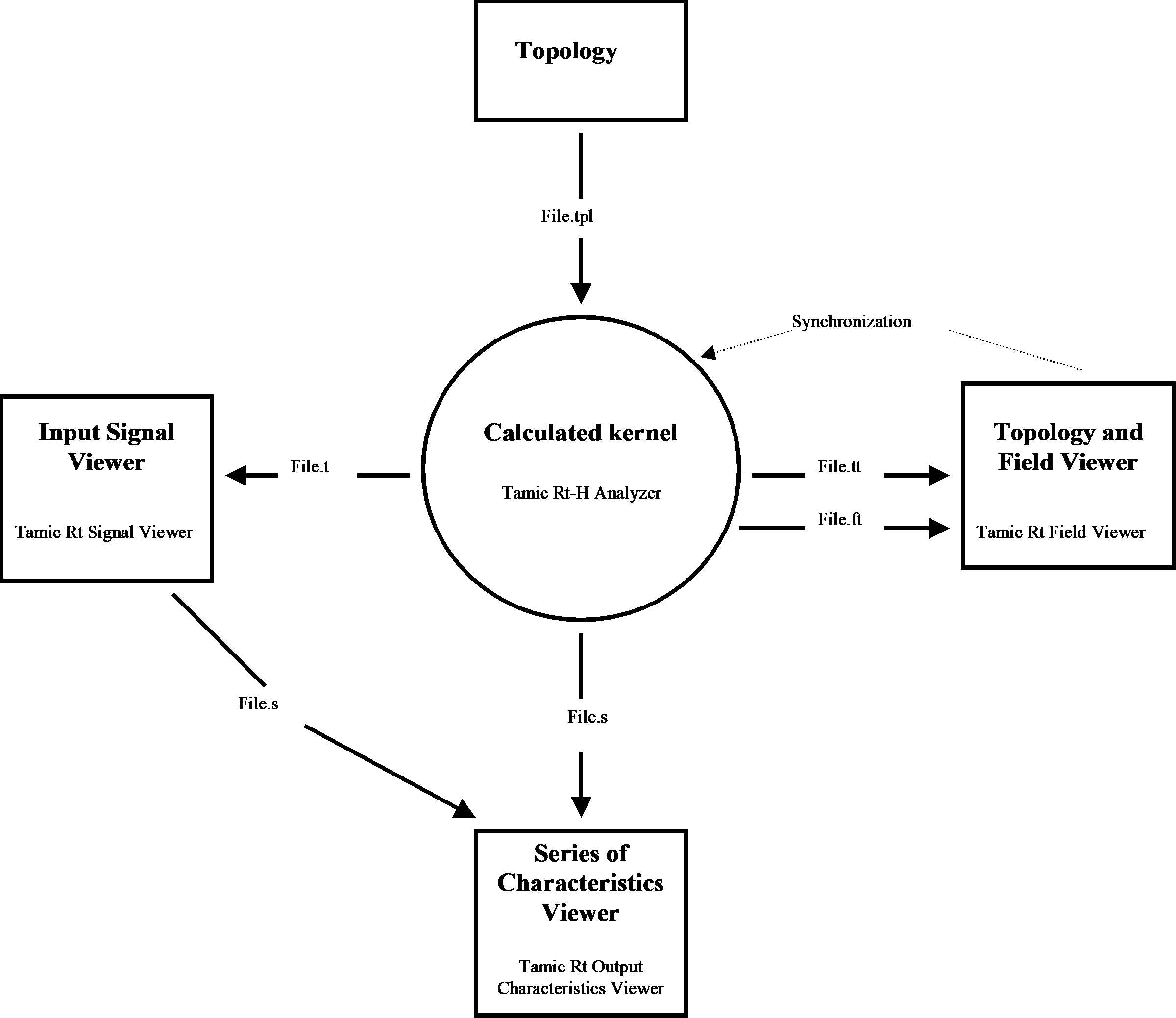
Структурная схема пакета (рис. 2.1 авторского руководства).
Расхождение с рисунком. На схеме 2000 года файл поля обозначен
File.ft, а в тексте того же руководства —File.tf. В текущем коде поле пишется в файлы.ex/.ey/.hz/.em/.ef(см. раздел 8). Расширение.tfосталось только в списке открываемых FieldView форматов.
Такое разделение (счёт отдельно, просмотр отдельно) позволяет повысить гибкость системы и минимизировать требования к ресурсам компьютера при проведении расчёта.
2. Общая структура файла задания
Каждая строка файла начинается уникальным описателем, который определяет следующие за ним данные.
Файл задания всегда начинается строкой #TMC_RT_H и заканчивается строкой #EOF.
Всё задание делится на шаги. Каждый шаг может описывать независимое СВЧ-устройство или его часть;
шаг начинается строкой #STEP и заканчивается #END_STEP:
#TMC_RT_H          Начало файла задания
#STEP              Это первый шаг
   Данные для первой задачи
#END_STEP
#STEP              Это второй шаг
   Данные для второй задачи
#END_STEP
#EOF               Конец файла задания
Сигнатура
#TMC_RT_H— общая для обоих ядер. X-ядро (tmc_rtx.exe) читает файлы с той же первой строкой#TMC_RT_H, отдельной сигнатуры#TMC_RT_Xв коде нет.
Каждый шаг состоит из четырёх секций, которые рекомендуется располагать в таком порядке:
| Секция | Назначение | Обязательна? |
|---|---|---|
#PARM … #END_PARM |
Единицы измерения, шаг сетки, время, границы «коробки», частота | В первом шаге — да |
#TOPOLOGY … #END_TOPOLOGY |
Блоки (графические примитивы), из которых состоит устройство | Да |
#LINK_LIST … #END_LINK |
Геометрическое положение каждого блока в «коробке» | Да |
#OUTPUT … #END_OUTPUT |
Какие выходные файлы формировать | Да (нужно хотя бы FILE) |
Секция параметров может отсутствовать в шагах, следующих за первым — тогда параметры берутся такими же, как в предыдущем шаге.
2.1. Синтаксис
- Все операторы, имеющие символ
#, должны начинаться с первой позиции строки. - Остальные операторы должны иметь как минимум один пробел в первой позиции строки.
- Комментарий — любая строка или часть строки, начинающаяся с символа
!. - Допустимы пустые строки и строки из одних пробелов.
- Параметры отделяются от идентификатора строки как минимум одним пробелом, а между собой —
символом
;.
В формализованных записях формата ниже приняты обозначения:
| Обозначение | Смысл |
|---|---|
< > |
обязательный параметр |
[ ] |
необязательный параметр |
expression |
математическое выражение |
expression(x,y,r,f) |
выражение, содержащее функцию от декартовых (x,y) или полярных (r,f) координат |
n |
целое число |
3. Методика: как составить задание с нуля
Это тот самый порядок действий, которым пользовался автор. Разберём его на задаче из авторского руководства: рассеяние плоской волны на плоскопараллельной пластине с ε = 4 на частоте 10 ГГц.
Шаг 1. Нарисовать топологию в H-плоскости
Начинают с чертежа реального устройства в H-плоскости, со всеми размерами.
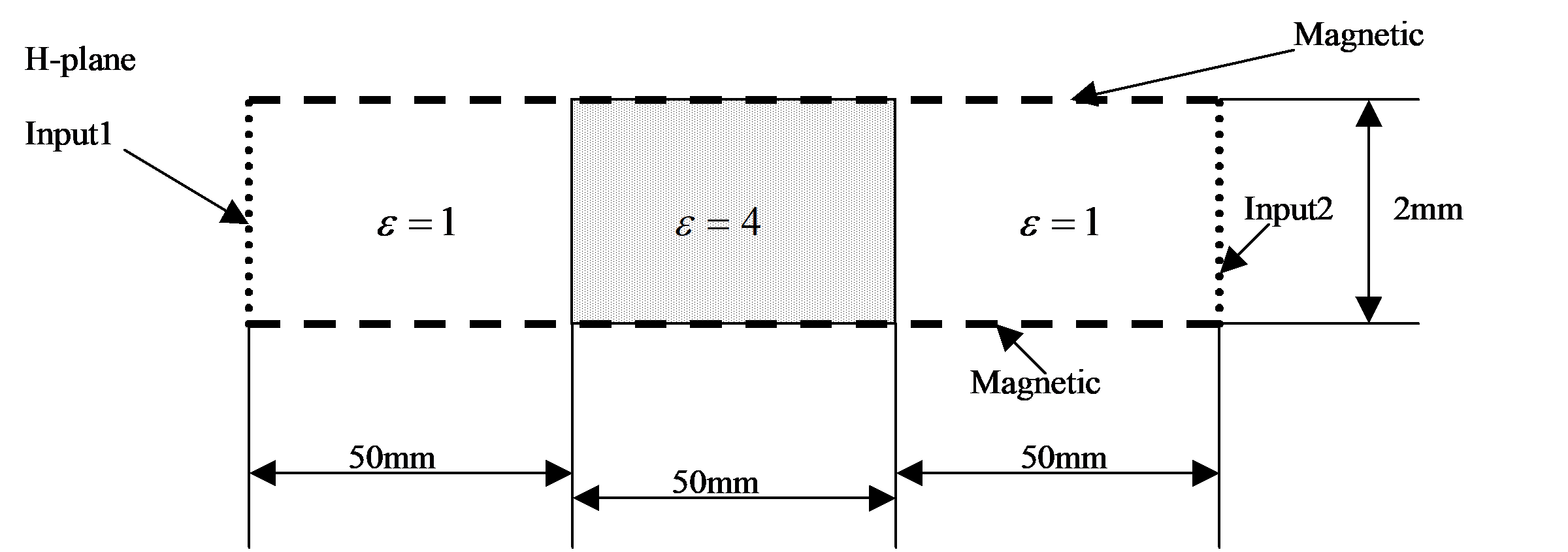
Расположение плоскопараллельной пластины в H-плоскости (рис. 3.1). Все размеры в миллиметрах.
Шаг 2. Вписать устройство в «коробку»
Всё устройство должно помещаться в прямоугольник — его называют «коробкой». Положение коробки
задаётся в секции параметров величинами X_MIN, X_MAX, Y_MIN, Y_MAX.
Границей коробки является металл или входы устройства. Это важно: сама граница коробки — всегда металл, если на ней не стоит вход.
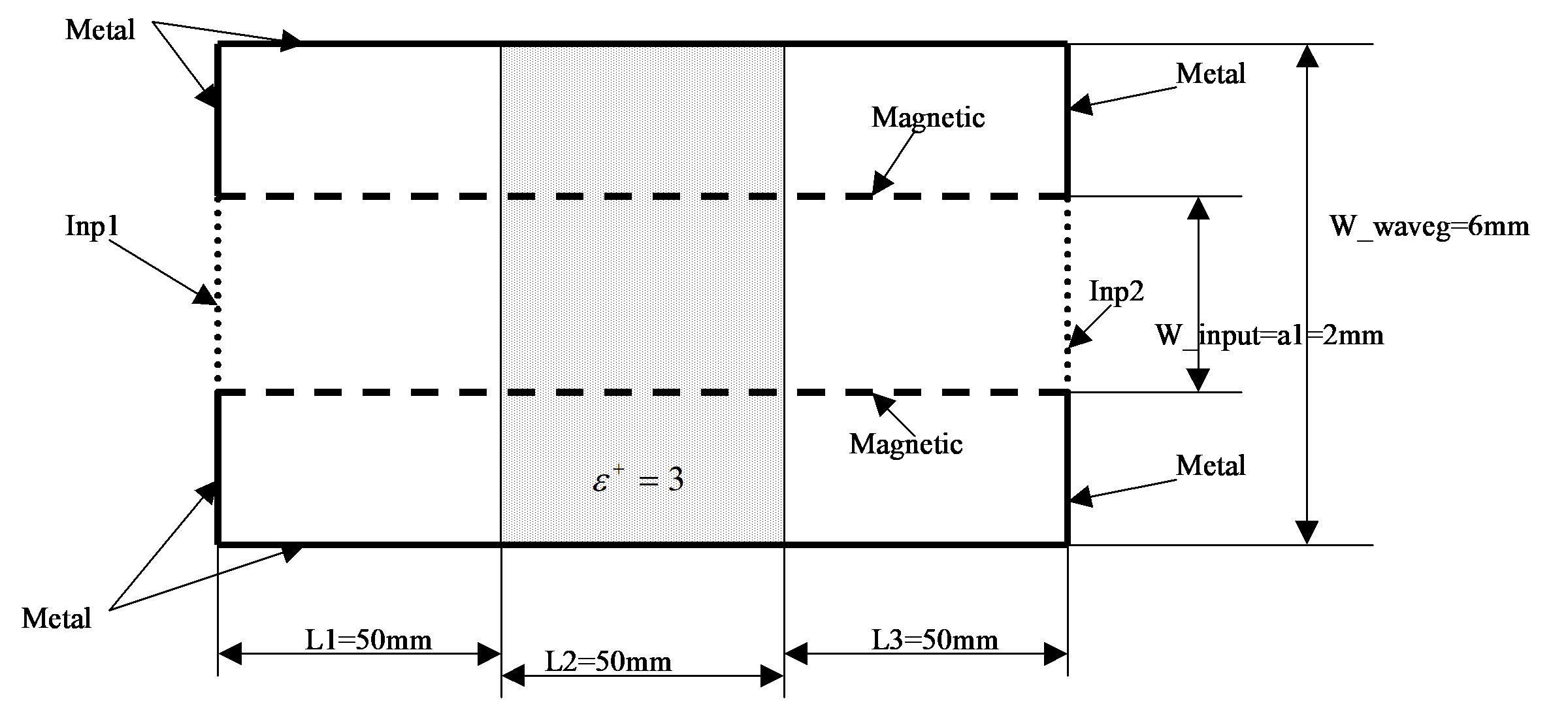
Расположение пластины в «коробке» и значения задаваемых константных выражений (рис. 3.2).
Обратите внимание на обозначение ε⁺ = 3 внутри пластины: это не сама проницаемость, а добавка к проницаемости вакуума. Пластине с ε = 4 соответствует добавка ε⁺ = 3 (см. раздел 5.1).
Шаг 3. Декомпозировать геометрию на примитивы
Полученную геометрию раскладывают на блоки — графические примитивы входного языка.
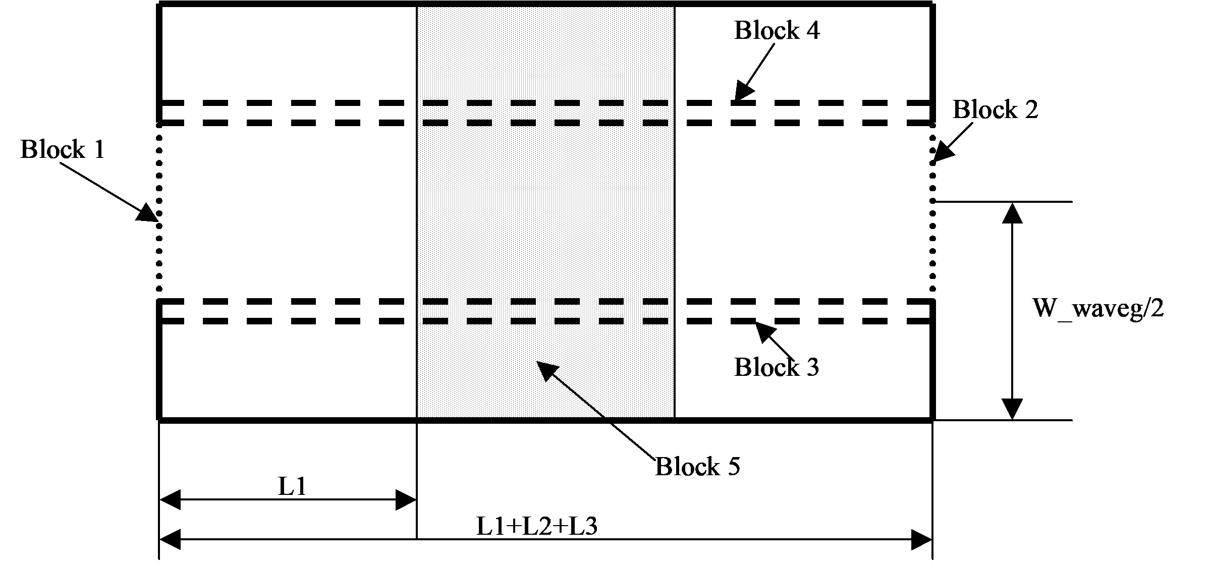
Декомпозиция заданной геометрии с использованием графических примитивов (рис. 3.3).
Для нашей задачи получается пять блоков:
| Блок | Что это |
|---|---|
| Block 1, Block 2 | входы устройства (INPUT_X) |
| Block 3, Block 4 | прямоугольники с магнитными стенками (RECT_STAT MAGNETIC) |
| Block 5 | прямоугольник с заданным диэлектрическим распределением (RECT_STAT) |
Шаг 4. Выбрать шаг сетки Δ
Шаг сетки DELTA определяет точность. Правила выбора — в разделе 4.5. Кратко: ориентировочно
1/20 длины волны в волноводе на максимальной частоте диапазона даёт точность около 3 %.
Шаг 5. Написать задание
Каждый блок описывается в секции #TOPOLOGY в своей локальной системе координат, а затем
размещается в коробке строкой T в секции #LINK_LIST.
Полный текст задания (файл samples/SAMPLE_R/TEST_MAG/EPS4/TEST0.TPL, приведён по авторскому
руководству — в репозитории файл с тех пор изменялся, см. примечание ниже):
#TMC_RT_H
#define L1 @ (   50.00)
#define L2 @ (   50.00)
#define L3 @ (   50.00)
#define W_freq @ (  10 )
#define W_eps @ ( 4.00 )
#define W_waveg @ (  6.00 )
#define W_input @ (  2.00 )
#define W_delta @ (    0.5 )
#define W_type @ MAGNETIC
#define a1 @ ( W_input )
#STEP
#PARM
 ANGLE_UNIT radian;
 FREQ_UNIT GHz;
 LONG_UNIT mm;
 TIME_UNIT ns;
 DELTA W_delta;
 TIME 0.; 5;
 X_MIN  0.0;
 X_MAX L1+L2+L3;
 Y_MIN  0.0;
 Y_MAX W_waveg;
 FREQ  10;
#END_PARM
#TOPOLOGY
 BLOCK 1;
  INPUT_X   W_type ; -a1/2; a1/2; 0; 200;
 END_B
 BLOCK 2;
  INPUT_X    W_type ; -a1/2; a1/2; 200; 201;
 END_B
 BLOCK 3;
  RECT_STAT W_type ; 0.0; L1+L2+L3; -a1/2-2*W_delta; -a1/2-1*W_delta;
 END_B
 BLOCK 4;
  RECT_STAT W_type ; 0.0;L1+L2+L3; a1/2; a1/2+W_delta;
 END_B
 BLOCK 5;
  RECT_STAT (W_eps-1); 0;L2; 0.0; W_waveg;
 END_B
#END_TOPOLOGY
#LINK_LIST
 T 1; 0.0; W_waveg/2;
 T 2; L1+L2+L3; W_waveg/2;
 T 3; 0.0; W_waveg/2;
 T 4; 0.0; W_waveg/2;
 T 5; L1; 0.0;
#END_LINK
#OUTPUT
 FILE test1;
 SMATRIX test1; 10; 4; 5;
 FIELDS;
 TOPOLOGY;
#END_OUTPUT
#END_STEP
#EOF
Разбор ключевых мест:
#define W_eps @ ( 4.00 )— проницаемость пластины ε = 4;RECT_STAT (W_eps-1); …— в блок передаётся добавка ε⁺ = ε − 1 = 3. Отсюда-1;INPUT_X W_type; -a1/2; a1/2; 0; 200;— вход ширинойa1, радиоимпульс с 0 по 200 нс;- второй вход (Block 2) имеет
T_min = 200, что больше времени анализа (TIME 0.; 5;) — так задают вход, на котором нет падающей волны, только приём; SMATRIX test1; 10; 4; 5;— записать S-матрицу для частоты 10 ГГц, усреднив с 4 по 5 нс.
Файл в репозитории отличается от руководства. В
samples/SAMPLE_R/TEST_MAG/EPS4/TEST0.TPLс 2000 года измененыL1=100,L2=600,L3=100,W_eps=-0.01,W_delta=0.1,TIME 0.; 200;, а у первого входа появились дополнительные параметры (… 0; 200; 1.; ;— амплитуда и фаза, см. раздел 6.4). Приведённый выше текст — из руководства; он показывает исходный замысел.
Шаг 6. Проверить и запустить
- Откройте
.tplв ядре (File → Open). - Ошибки разбора выводятся с указанием строки — язык проверяется строго.
- Запустите расчёт и посмотрите результаты вьюверами (раздел 8).
4. Секция параметров #PARM
#PARM
    . . .
#END_PARM
#PARMили#PARMS? В авторском руководстве 2000 года разделы «Формат ввода» пунктов 4.1.x написаны через#PARMS/#END_PARMS(11 мест), а все реальные примеры и оглавление — через#PARM/#END_PARM. Это след родственного продукта TAMIC-E/H, где секция действительно называется#PARMS.Оба варианта работают. Канонические имена в коде —
#PARMи#END_PARM(src/Include/TmcRTH_Indan.h, строка 23), но секции ищутся сравнением по префиксу (strncmp(csCh, csSection, csSection.GetLength())вTmcRTH_Indan.cpp, строки 435 и 460), поэтому#PARMSи#END_PARMSтоже совпадают. Рекомендуется писать#PARM/#END_PARM.
Единицы измерения углов, частоты, длин и времени необходимо задавать до определения частот и параметров с размерностью длины и времени.
Секция обязательно должна присутствовать в первом шаге. Если в других шагах она отсутствует, то параметры будут такими, как в предыдущем шаге.
4.1. ANGLE_UNIT — единицы измерения углов
ANGLE_UNIT <radian> | <gradus>;
Фиксирует единицу измерения углов аргументов тригонометрических функций.
| Значение | Смысл |
|---|---|
radian |
радианы |
gradus |
градусы |
По умолчанию — как в предыдущем шаге; если шаг первый — radian.
4.2. FREQ_UNIT — единицы измерения частоты
FREQ_UNIT <GHz> | <MHz> | <kHz> | <Hz>;
Вводится до строки FREQ. По умолчанию в первом шаге — GHz.
4.3. LONG_UNIT — единицы измерения длины
LONG_UNIT <mm> | <cm> | <m>;
Вводится до строк DELTA, X_MIN, X_MAX, Y_MIN, Y_MAX. По умолчанию в первом шаге — mm.
4.4. TIME_UNIT — единицы измерения времени
TIME_UNIT <s> | <ms> | <mks> | <ns> | <ps>;
Вводится до строки TIME.
По авторскому руководству, значение по умолчанию в первом шаге — секунды (
s), а неns. Единицу времени лучше задавать явно.
4.5. DELTA — шаг сетки (точность анализа)
DELTA <expression>;
Физический смысл — размер пространственного дискрета, шага квадратной сетки, на которую разбивается всё устройство. Это главный параметр точности.
Рекомендации автора:
- Для точности около 3 % величина должна составлять около 1/20 длины волны в волноводе на максимальной частоте диапазона. Точнее — определяется серией расчётов на сходимость.
- При уменьшении шага время анализа растёт пропорционально кубу. Поэтому первоначальную отработку устройства ведут при низкой точности, повышая её на заключительном этапе.
- Подбирайте шаг и геометрию так, чтобы геометрия вписывалась целым числом дискретов. Если
толщина металла 1, 2, 3, 4 мм — берите
DELTA= 1 мм или 0.5 мм, а не 1.02 мм или 0.47 мм. - Время счёта минимально, если в «коробке» вдоль X и Y укладывается целое число дискретов.
В первом шаге параметр обязателен.
4.6. TIME — время анализа
TIME <expression>; <expression>;
Первый параметр — время начала анализа, второй — время окончания. В первом шаге обязателен.
4.7. X_MIN, X_MAX, Y_MIN, Y_MAX — границы «коробки»
X_MIN <expression>;
X_MAX <expression>;
Y_MIN <expression>;
Y_MAX <expression>;
Задают прямоугольник, в который помещается анализируемая топология. В первом шаге обязательны.
4.8. FREQ — частота сигналов возбуждения
FREQ <expression>;
Частота сигналов возбуждения на входах устройства. В первом шаге обязателен.
4.9. Параметры, принимаемые кодом, но не влияющие на расчёт
Разбор этих строк в коде есть, значение сохраняется, но ни одно ядро его не читает. Проверено по
исходникам: соответствующие геттеры (dGetHeight, GetDeltaT, IsDeltaTDefine) не вызываются ни из
kernels/, ни из fieldview/, ни из viewers/; поля rNUnit / rBUnit не читаются вне модуля
разбора.
| Ключевое слово | Формат | Состояние |
|---|---|---|
HEIGHT |
HEIGHT <expression>; |
Разбирается, на расчёт не влияет. Встречается в samples/SAMPLE_R/TEST_*/…/HWVGD_1.TPL (HEIGHT 0.1;) |
DELTA_T_MECHANICAL |
DELTA_T_MECHANICAL <expression>; |
Разбирается, вызывает SetDeltaT(), но результат не читается |
N_UNIT |
N_UNIT <m3> \| <cm3> \| <mm3>; |
Разбирается, множитель не применяется |
B_UNIT |
B_UNIT <Tl> \| <mTl> \| <mkTl>; |
Разбирается, множитель не применяется |
Практическое следствие: концентрация плазмы N в блоках *_STAT_N всегда трактуется в м⁻³,
а индукция B в блоках *_STAT_B — всегда в Тесла, независимо от того, что написано в
N_UNIT / B_UNIT.
5. Секция топологии #TOPOLOGY
#TOPOLOGY
    BLOCK 1;
        <тип примитива и его параметры>
    END_B
    . . .
    BLOCK <n>;
        . . .
    END_B
#END_TOPOLOGY
Каждому блоку присваивается уникальный номер <n> — целое число больше нуля. Номера не
обязаны идти по порядку и не обязаны быть непрерывными (в авторском примере с рупорами
используются номера 1, 2, 5, 6, 7, 12, 14, 21, 22, 25, 26, 41…46, 104).
Параметры каждого примитива описываются в его локальной системе координат. Положение блока в
коробке определяется в #LINK_LIST — поэтому каждому блоку обязательно должна соответствовать
одна строка в #LINK_LIST.
Все примитивы, кроме входов (INPUT_X, INPUT_Y), могут накладываться и пересекаться между собой.
Входы обязательно должны помещаться только на границе «коробки».
5.1. Материал или распределение ε
Первый параметр примитива задаёт либо материал, либо распределение добавки диэлектрической проницаемости:
| Значение | Смысл |
|---|---|
METAL |
металл (идеальный проводник) |
MAGNETIC |
магнетик — стенка холостого хода (магнитная стенка) |
ABSORBER |
поглотитель |
expression(x,y,r,f) |
распределение добавки ε⁺ к проницаемости вакуума |
Ключевое соглашение: задаётся добавка, а не сама проницаемость.
| Нужная ε | Что писать |
|---|---|
| ε = 4 | 3 |
| ε = 9 | 8 |
| ε = 1 (вакуум) | 0 |
| ε = 0 | -1 |
| ε = 0.25 | -0.75 |
Важная разница в смысле примитива — материал задаёт КОНТУР, а не заливку. Если задан материал, примитив задаёт границу (контур, ломаную линию). Если задано выражение, примитив задаёт область, заполненную средой. Это хорошо видно на рисунках ниже: у
RECT_STAT METALметаллом является только контур прямоугольника, а уRECT_STAT 8закрашена вся площадь.Подтверждено кодом:
SetRectMetal(src/kernels/PlanarRT_H/TmcRTHNodeDiel.cpp:2419) выделяетnNumNode = 2*nX + 2*(nY-1)узлов — это периметр, а неnX*nY(заливка), и заполняет их четырьмя циклами: нижнее ребро (y = dYmin), верхнее (y = dYmax), левое (x = dXmin), правое (x = dXmax).Практическое следствие. Чтобы получить сплошной металлический объект, задавайте его контуром: поле внутрь замкнутого контура не проникает. А чтобы получить сплошную диэлектрическую вставку — задавайте выражение, оно заполняет площадь.
Внимание,
METALиMAGNETICменяются местами. Вsrc/Include/Tmcgrviw.h(строки 159–165) определения зависят от макроса_MODEL_RTE__: при его наличииMETALиMAGNETICменяются ролями (модель E-плоскости). В штатных сборках H и X этот макрос не задаётся, и слова означают то, что написано.
5.2. RECT_STAT — неподвижный прямоугольник
BLOCK <n>;
    RECT_STAT [[file_name]]<METAL> | <MAGNETIC> | <ABSORBER> | <expression(x,y,r,f)>;
    <X_min>; <X_max>;
    <Y_min>; <Y_max>;
END_B
| № | Параметр | Смысл |
|---|---|---|
| 1 | материал / выражение | см. раздел 5.1 |
| 2 | X_min |
левая граница по X |
| 3 | X_max |
правая граница по X |
| 4 | Y_min |
нижняя граница по Y |
| 5 | Y_max |
верхняя граница по Y |
Необязательный [file_name] в квадратных скобках перед выражением — сохранить рассчитанное
распределение ε в файл file_name.eps, чтобы потом переиспользовать его примитивом FILE
(раздел 5.6). Нужно для повышения эффективности при повторении вычислений на больших площадях.
Два дополнительных условия для MAGNETIC и ABSORBER:
- Разности
X_max − X_minиY_max − Y_minдолжны превышать2*DELTA— толщина и высота должны быть больше двух пространственных дискретов. - Весь прямоугольник должен находиться в коробке, и его граница должна отстоять от границы коробки не менее чем на один шаг сетки.
Примеры
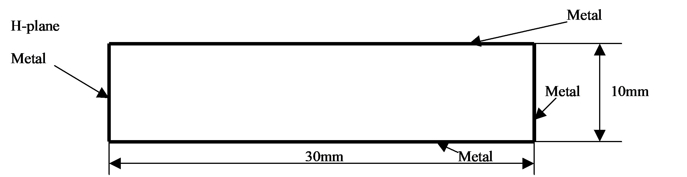
Рис. 4.1. Неподвижный прямоугольник 30×10 мм, ограниченный металлом.
BLOCK 1;
    RECT_STAT METAL; 0; 30; 0; 10;
END_B
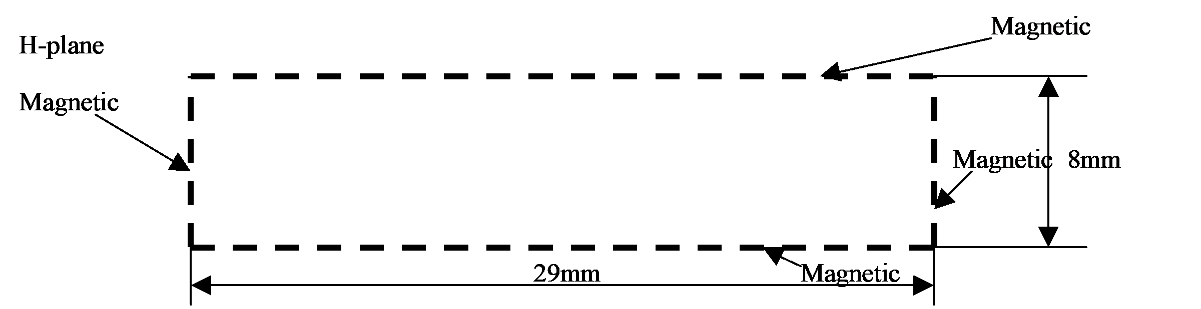
Рис. 4.2. Прямоугольник 29×8 мм со стенками холостого хода (магнетиком).
BLOCK 1;
    RECT_STAT MAGNETIC; -29; 0; -8; 0;
END_B
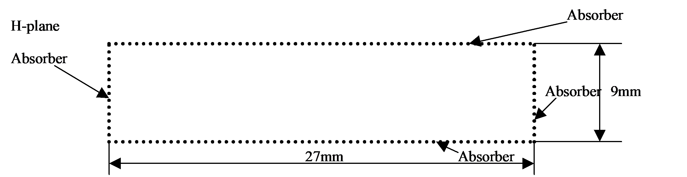
Рис. 4.3. Прямоугольник 27×9 мм с поглощающими стенками.
BLOCK 1;
    RECT_STAT ABSORBER; 0; 27; 0; 9;
END_B
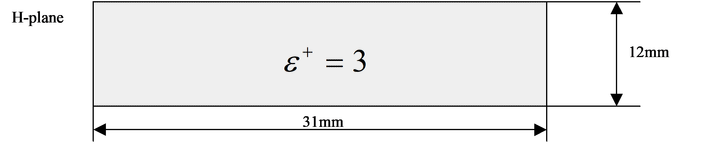
Рис. 4.4. Прямоугольник 31×12 мм с ε = 4 (добавка ε⁺ = 3).
BLOCK 1;
    RECT_STAT 3; 0; 31; 0; 12;
END_B
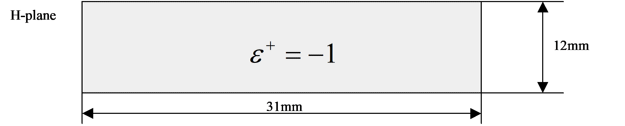
Рис. 4.5. Прямоугольник 31×12 мм с ε = 0 (добавка ε⁺ = −1).
BLOCK 1;
    RECT_STAT -1; 0; 31; 0; 12;
END_B
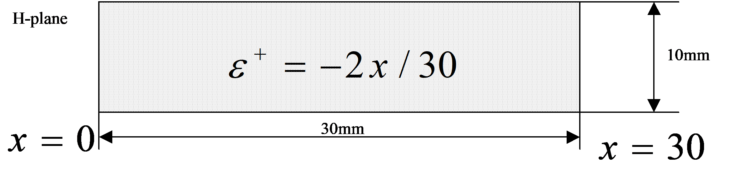
Рис. 4.6. Прямоугольник 30×10 мм, ε линейно падает вдоль X от 1 на левой границе до −1 на правой (добавка меняется от 0 до −2).
BLOCK 1;
    RECT_STAT -2*x/30; 0; 30; 0; 10;
END_B
5.3. CIRCLE_STAT — неподвижный сектор
BLOCK <n>;
    CIRCLE_STAT <METAL> | <MAGNETIC> | <ABSORBER> | <expression(x,y,r,f)>;
    <R_min>; <R_max>;
    <F_min>; <F_max>;
END_B
| № | Параметр | Ограничение |
|---|---|---|
| 1 | материал / выражение | см. раздел 5.1 |
| 2 | R_min |
≥ 0 |
| 3 | R_max |
> R_min |
| 4 | F_min |
≥ 0 |
| 5 | F_max |
> F_min, ≤ 2π |
R_min, R_max — в единицах LONG_UNIT; F_min, F_max — в единицах ANGLE_UNIT.
Примеры
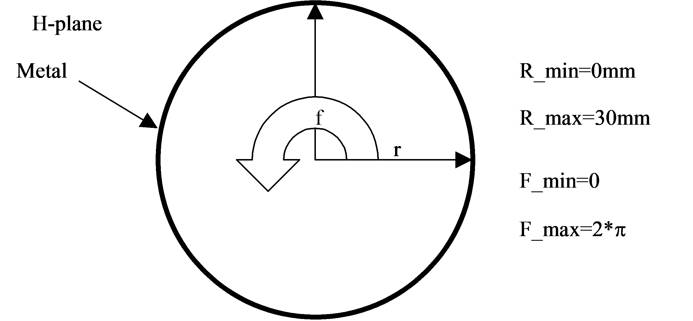
Рис. 4.7. Металлический круг радиусом 30 мм.
BLOCK 1;
    CIRCLE_STAT METAL; 0; 30; 0; 2*3.141592653589;
END_B
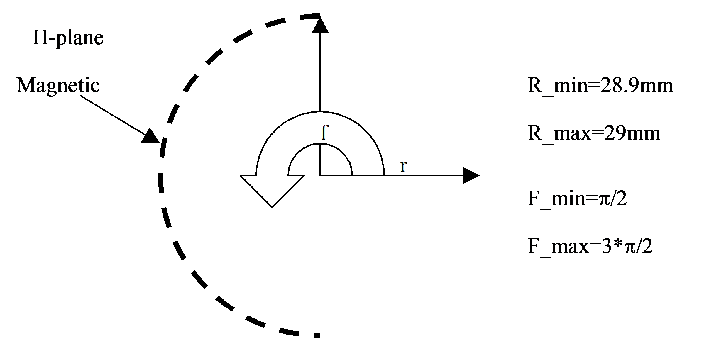
Рис. 4.8. Полуокружность из магнетика радиусом 29 мм.
BLOCK 1;
    CIRCLE_STAT MAGNETIC; 28.9; 29; 3.141592653589/2; 3*3.141592653589/2;
END_B
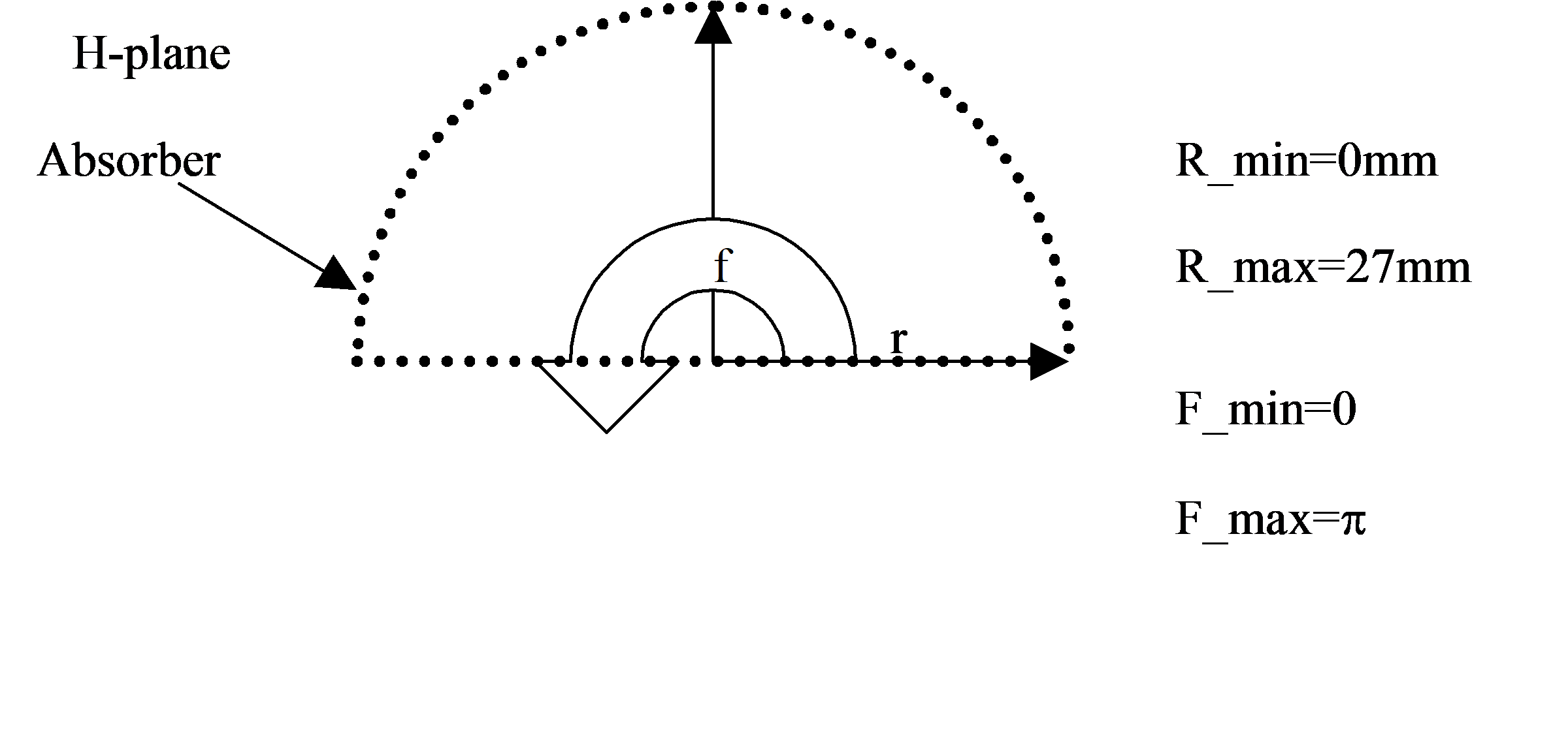
Рис. 4.9. Полукруг из поглотителя радиусом 27 мм.
BLOCK 1;
    CIRCLE_STAT ABSORBER; 0; 27; 0; 3.141592653589;
END_B
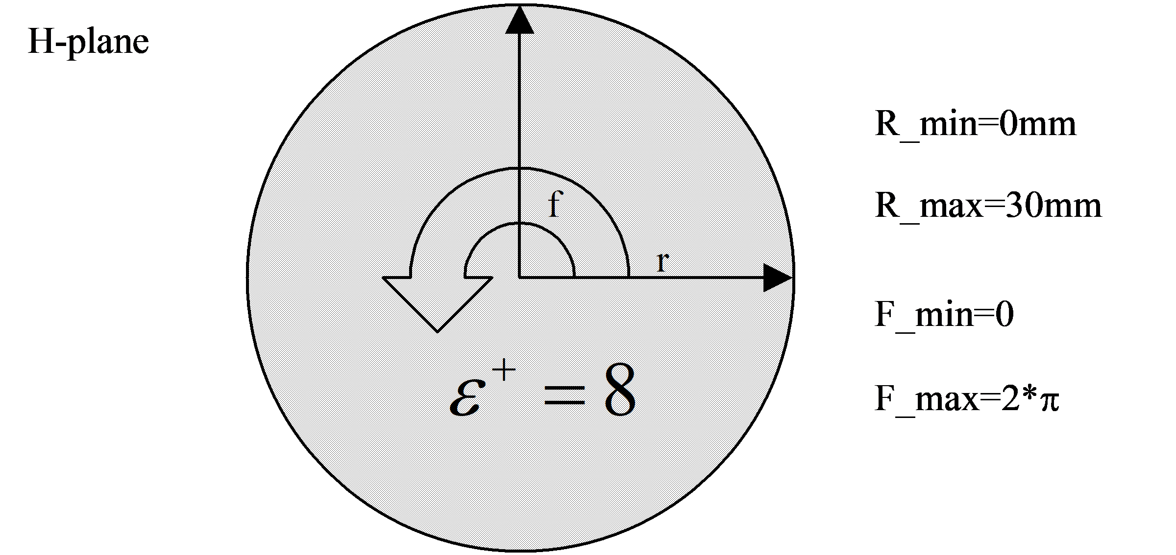
Рис. 4.10. Круг радиусом 30 мм с ε = 9 (добавка ε⁺ = 8).
BLOCK 1;
    CIRCLE_STAT 8; 0; 30; 0; 2*3.141592653589;
END_B
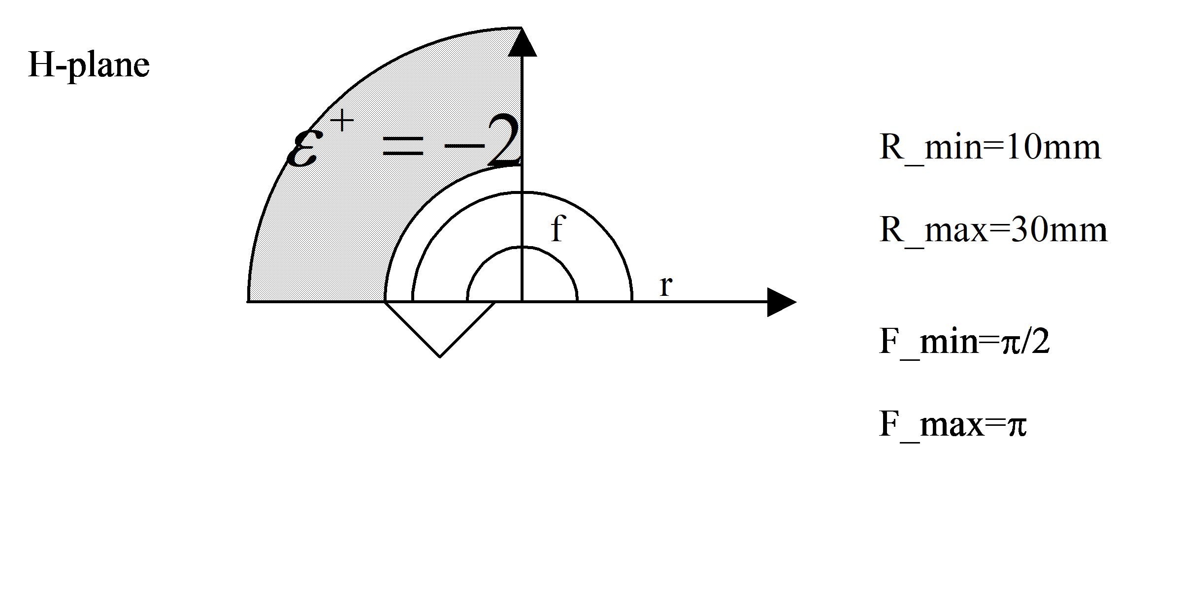
Рис. 4.11. Сектор с ε = −1 (добавка ε⁺ = −2).
BLOCK 1;
    CIRCLE_STAT -2; 10; 30; 3.141592653589/2; 3.141592653589;
END_B
5.4. POLYGON_STAT — неподвижный многоугольник
BLOCK <n>;
    POLYGON_STAT <METAL> | <MAGNETIC> | <ABSORBER> | <expression(x,y,r,f)>;
        L <expression>; <expression>;
        L <expression>; <expression>;
        L <expression>; <expression>;
        [L <expression>; <expression>;]
        …
END_B
В первой строке — материал или выражение. В последующих строках после символа L вводятся абсцисса
и ордината вершины в локальной системе координат блока.
Поведение зависит от первого параметра — это важно:
| Первый параметр | Поведение |
|---|---|
| выражение (ε) | Последняя точка соединяется с первой, образуя замкнутую область. Область должна быть односвязной и выпуклой, вершины обходятся по часовой стрелке. Число вершин должно быть больше 3. |
METAL, MAGNETIC, ABSORBER |
Последняя точка не соединяется с первой — формируется ломаная линия, а не замкнутая область. Направление обхода и выпуклость соблюдать не нужно. |
Программа не контролирует, является ли область замкнутой и односвязной, а также правильность направления обхода вершин. Ошибка здесь не диагностируется — она проявится как неверный результат.
Примеры
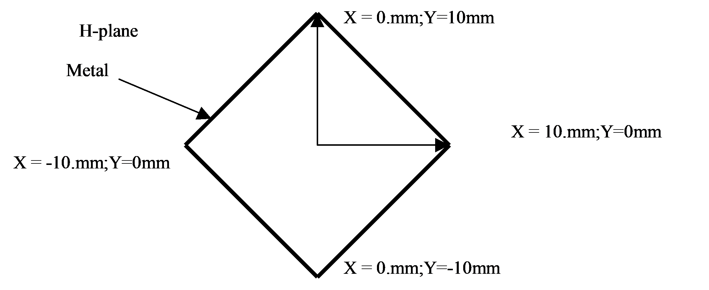
Рис. 4.12. Металлический четырёхугольник (замкнут явно — первая точка повторена в конце).
BLOCK 1;
    POLYGON_STAT METAL;
        L -10; 0;
        L 0; 10;
        L 10; 0;
        L 0; -10;
        L -10; 0;
END_B
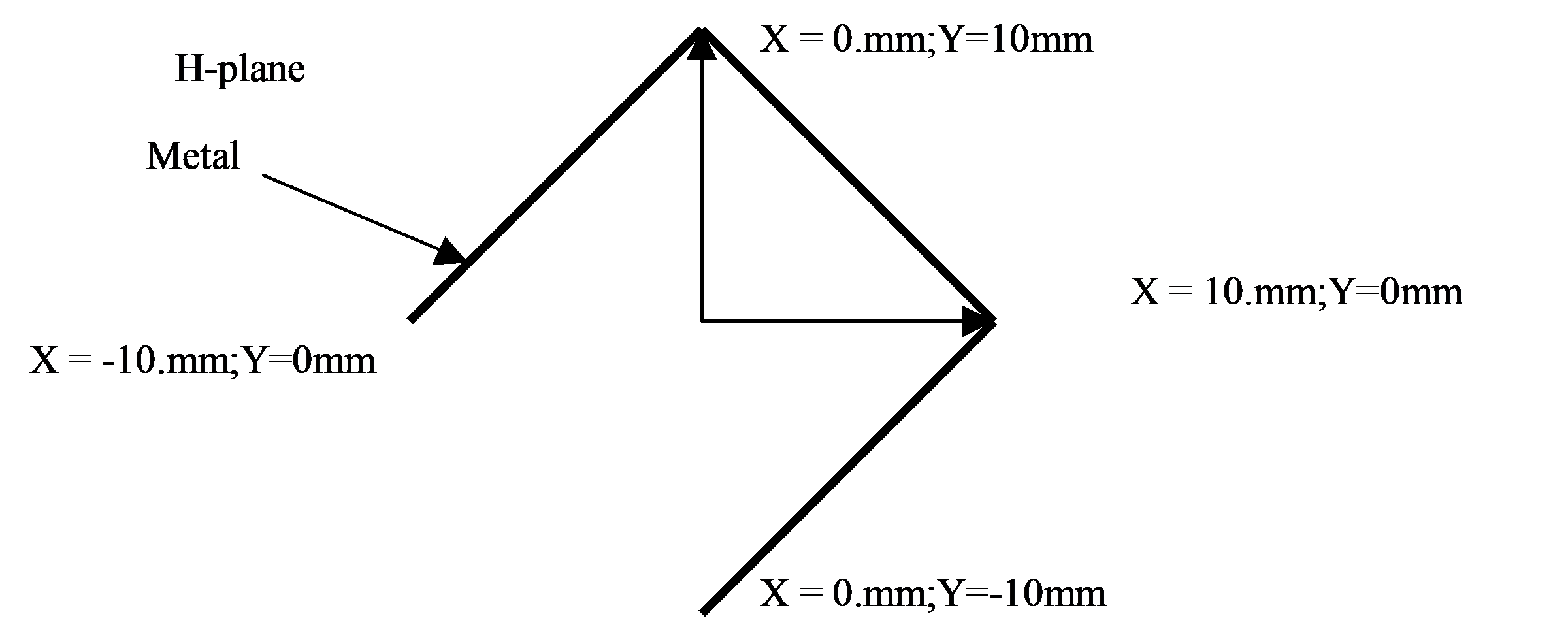
Рис. 4.13. Металлическая ломаная линия (та же запись без повтора первой точки).
BLOCK 1;
    POLYGON_STAT METAL;
        L -10; 0;
        L 0; 10;
        L 10; 0;
        L 0; -10;
END_B
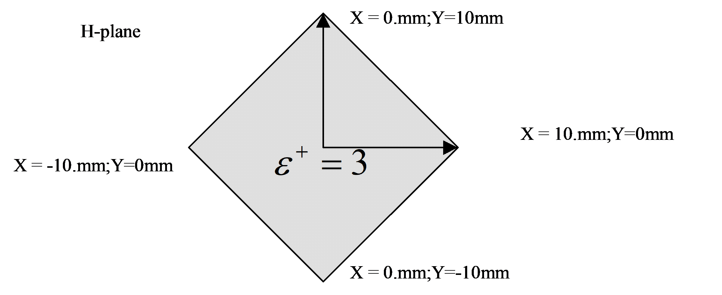
Рис. 4.14. Диэлектрический четырёхугольник с ε = 4 (добавка ε⁺ = 3) — область замыкается сама.
BLOCK 1;
    POLYGON_STAT 3;
        L -10; 0;
        L 0; 10;
        L 10; 0;
        L 0; -10;
END_B
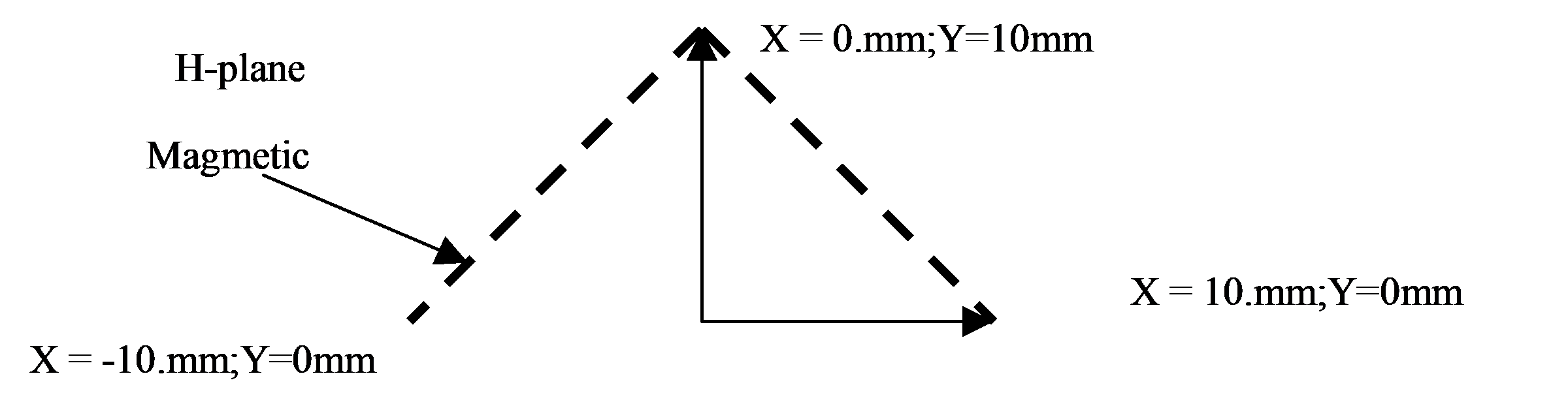
Рис. 4.15. Ломаная линия из магнитной стенки.
BLOCK 1;
    POLYGON_STAT MAGNETIC;
        L -10; 0;
        L 0; 10;
        L 10; 0;
END_B
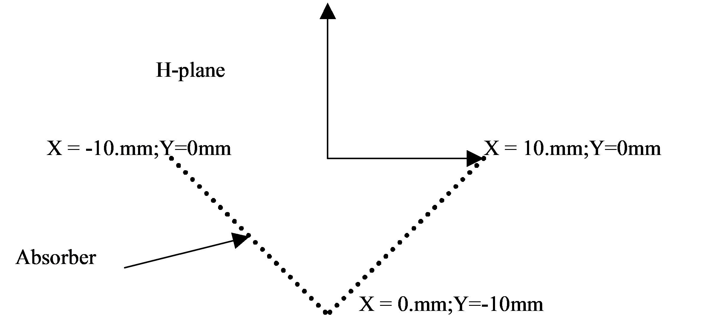
Рис. 4.16. Ломаная линия из поглотителя.
BLOCK 1;
    POLYGON_STAT ABSORBER;
        L 10; 0;
        L 0; -10;
        L -10; 0;
END_B
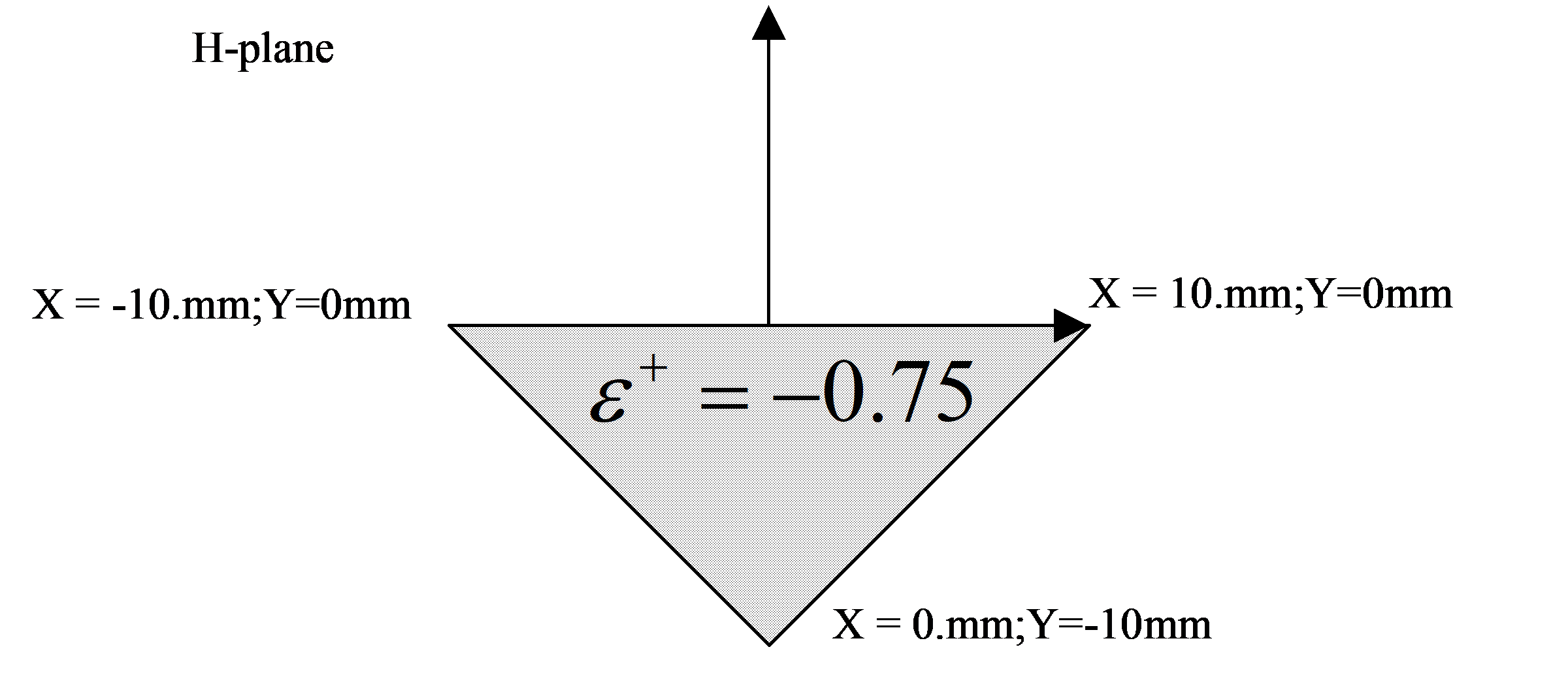
Рис. 4.17. Диэлектрический треугольник с ε = 0.25 (добавка ε⁺ = −0.75).
BLOCK 1;
    POLYGON_STAT -0.75;
        L 10; 0;
        L 0; -10;
        L -10; 0;
END_B
5.5. INPUT_X и INPUT_Y — входы (трансформаторы возбуждения)
По функциональному назначению блоки делятся на два типа: трансформаторы возбуждения и внутренние области. Все примитивы выше — внутренние области.
Осторожно с названиями — они означают не то, что кажется.
INPUT_X— это вход вдоль оси Y, он ставится на левую или правую границу коробки, и его размеры задаются по Y.INPUT_Y— это вход вдоль оси X, он ставится на нижнюю или верхнюю границу коробки, и его размеры задаются по X. На какой именно границе окажется вход, определяется координатами в#LINK_LIST.
BLOCK <n>;
    INPUT_X [<METAL> | <MAGNETIC>];
    <Y_min>; <Y_max>;
    <T_min>; <T_max>;
    [<Amplitude>]; [<Faza>];
    [<Eps>];
END_B
BLOCK <n>;
    INPUT_Y [<METAL> | <MAGNETIC>];
    <X_min>; <X_max>;
    <T_min>; <T_max>;
    [<Amplitude>]; [<Faza>];
    [<Eps>];
END_B
Параметры 1–5 (документированы в руководстве 2000 года):
| № | Параметр | Смысл |
|---|---|---|
| 1 | тип | Мода падающей волны (см. таблицу ниже) |
| 2 | Y_min / X_min |
Нижняя (левая) граница входа |
| 3 | Y_max / X_max |
Верхняя (правая) граница входа, > min |
| 4 | T_min |
Время начала радиоимпульса возбуждения |
| 5 | T_max |
Время окончания радиоимпульса возбуждения, > T_min |
Мода возбуждения задаётся первым параметром:
| Значение | Мода | Требование к ширине входа |
|---|---|---|
MAGNETIC |
плоская волна | ширина меньше половины длины волны входного сигнала |
METAL или пусто |
первый тип колебаний прямоугольного волновода (волна H₁₀) | ширина больше половины, но меньше полной длины волны |
Эти условия необходимо соблюдать, чтобы во входном сечении реализовывался одномодовый режим возбуждения и согласования. Мода, по которой смотрится отражённый сигнал, соответствует падающей.
Частота радиоимпульса определяется параметром FREQ из секции параметров.
Как задать вход без падающей волны (только приёмный). Если на входе отсутствует падающая волна,
T_minдолжно быть больше времени анализа из секции параметров (TIME). Именно так сделан второй вход в примере раздела 3:TIME 0.; 5;приINPUT_X …; 200; 201;.
Параметры 6–8 — расширение, которого нет в руководстве 2000 года.
Установлено по исходному коду (ReadInputX / ReadInputY в
src/libs/TMCIndan/TmcRTH_BolckList.cpp; вычисление — dAmplitude, dFaza,
CalculateYForInput в src/kernels/PlanarRT_H/TmcRTHNodeDiel.cpp):
| № | Параметр | Смысл | Если не задан |
|---|---|---|---|
| 6 | Amplitude |
Амплитуда сигнала — выражение от переменных t (текущее время) и f (частота) |
1.0 |
| 7 | Faza |
Фаза сигнала — выражение от t и f, в единицах ANGLE_UNIT |
0.0 |
| 8 | Eps |
Добавка ε в сечении входа (влияет на волновую проводимость входа) | не применяется |
Все три необязательны, но параметр 7 обязателен, если задан параметр 6 (иначе — ошибка
«Missing separator ';'»). Пустое значение допустимо: … 0; 200; 1.; ; означает амплитуду 1.0 и
фазу по умолчанию — именно так записан первый вход в текущем
samples/SAMPLE_R/TEST_MAG/EPS4/TEST0.TPL.
Переменные t и f позволяют задать огибающую импульса вместо прямоугольного радиоимпульса —
например, гауссову.
Примеры
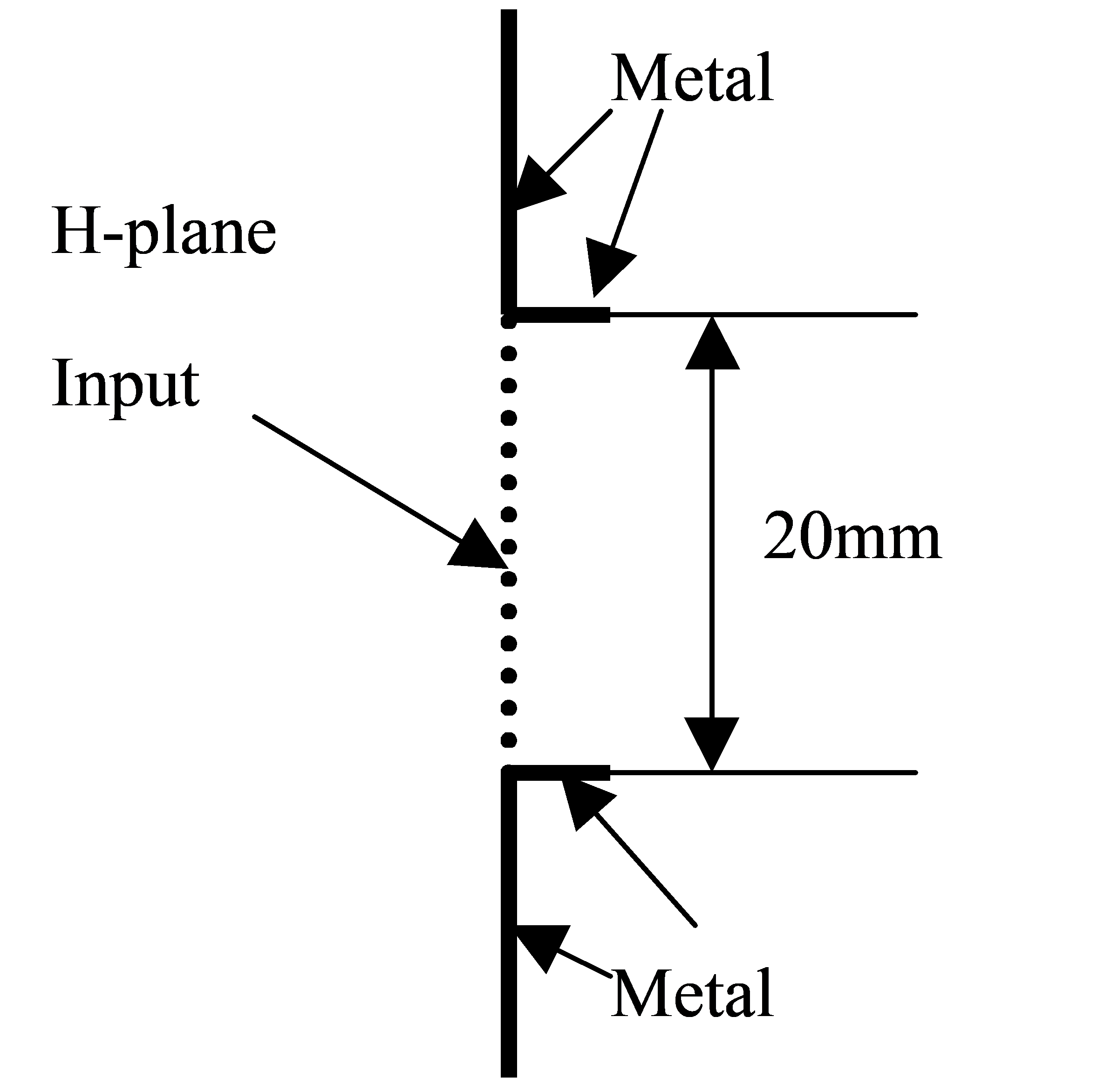
Рис. 4.18. Волноводный вход (H₁₀) шириной 20 мм, возбуждает систему радиоимпульсом длиной 10 нс.
BLOCK 1;
    INPUT_X METAL; 0; 20; 0; 10;
END_B
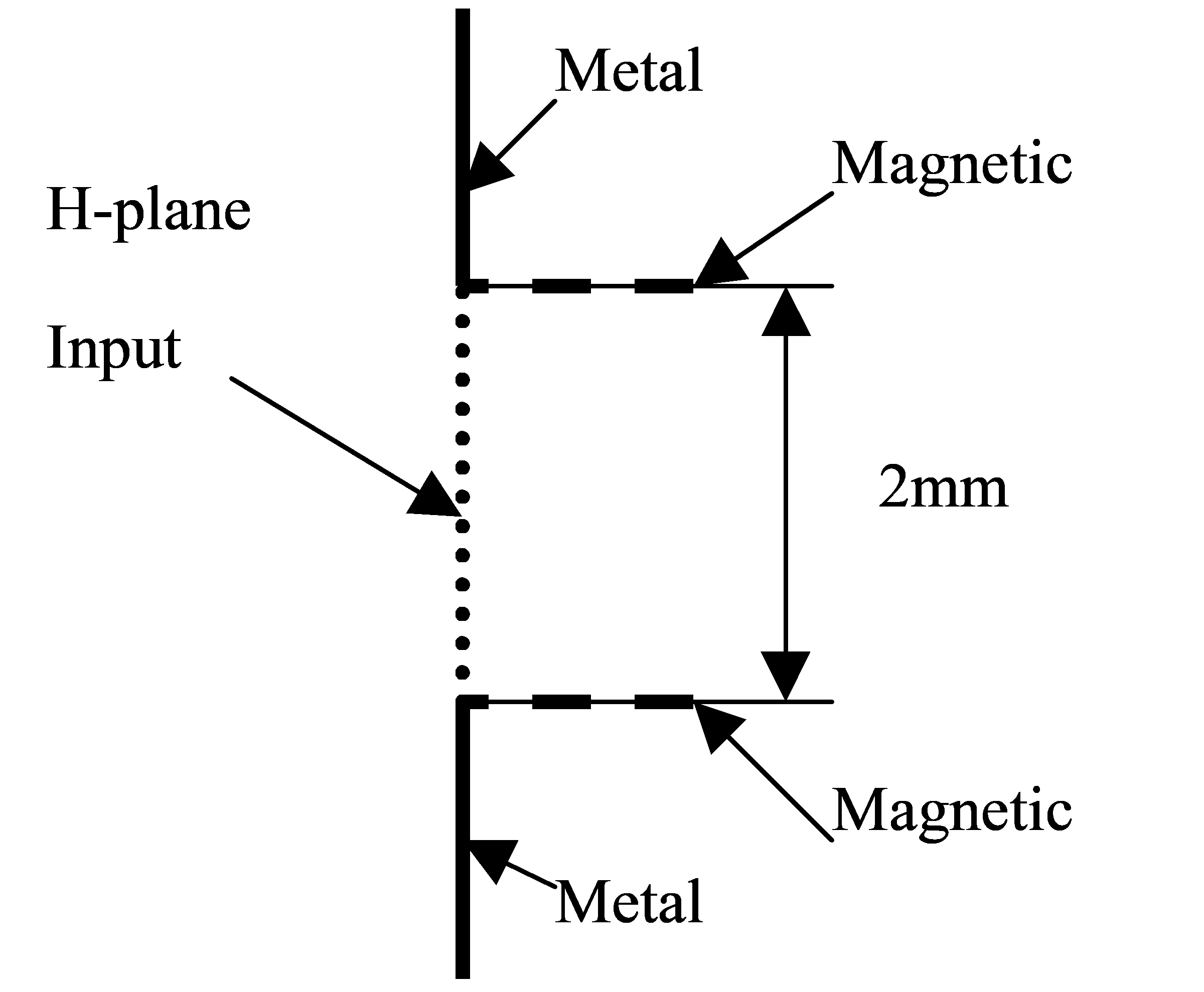
Рис. 4.19. Вход для плоской волны шириной 2 мм, радиоимпульс длиной 100 нс.
BLOCK 1;
    INPUT_X MAGNETIC; 0; 2; 0; 100;
END_B
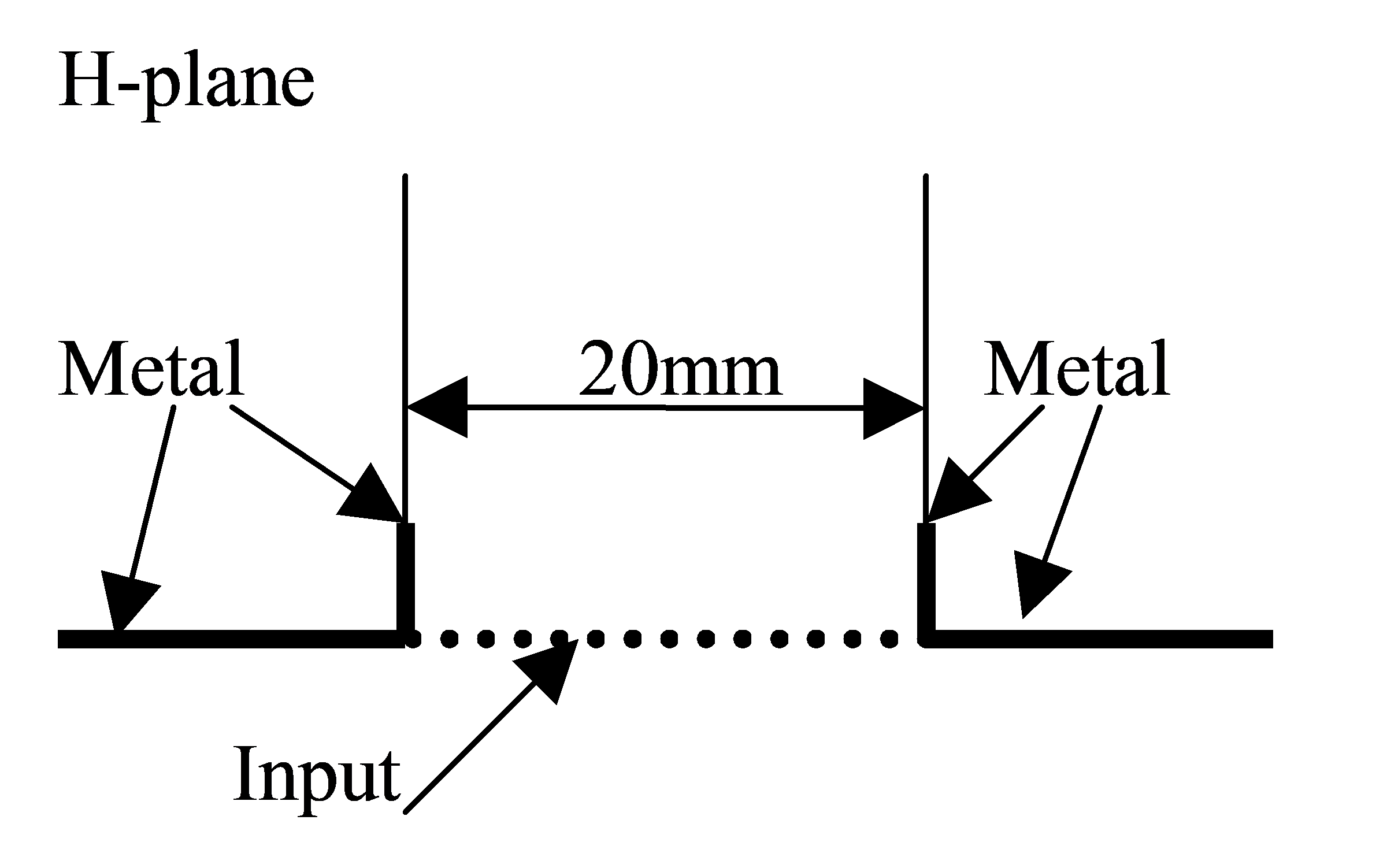
Рис. 4.20. Волноводный вход (H₁₀) шириной 20 мм вдоль оси X. Тип не указан — эквивалент METAL.
BLOCK 1;
    INPUT_Y ; 0; 20; 0; 10;
END_B
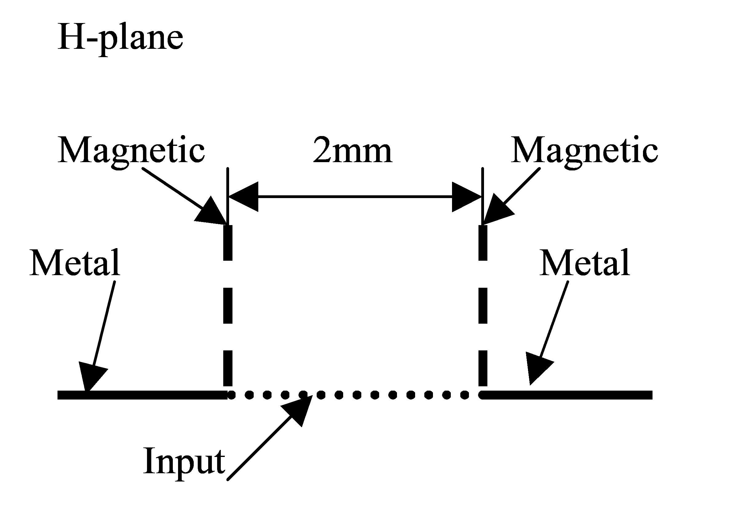
Рис. 4.21. Вход для плоской волны шириной 2 мм вдоль оси X.
BLOCK 1;
    INPUT_Y MAGNETIC; 0; 2; 0; 100;
END_B
5.6. FILE — чтение распределения ε из файла
BLOCK <n>;
    FILE <file_name>;
    <X_min>; <X_max>;
    <Y_min>; <Y_max>;
END_B
При расчёте распределения ε для больших площадей прямоугольников вычисление формулы в каждом узле
занимает заметное время. Его можно проделать один раз, сохранив результат в файл (параметр
[file_name] у RECT_STAT, раздел 5.2), а затем подставлять готовое распределение.
| № | Параметр | Смысл |
|---|---|---|
| 1 | file_name |
Имя файла с распределением. Должен находиться в той же директории, что и файл задания |
| 2–5 | X_min, X_max, Y_min, Y_max |
Границы прямоугольника |
Величины
X_min,X_max,Y_min,Y_maxдолжны быть такими же, как уRECT_STAT, из которого формировался файл.
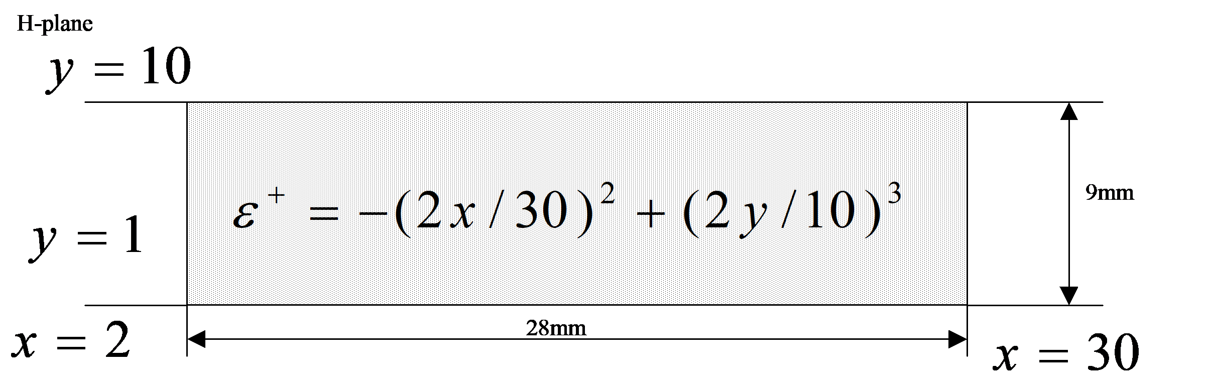
Рис. 4.22. Прямоугольник 30×10 мм, добавка ε⁺ задана функцией декартовых координат.
Сначала сохраняем распределение (первый шаг задания):
BLOCK 1;
    RECT_STAT [distr]-(2*x/30)^2+(2*y/10)^3; 2; 30; 1; 10;
END_B
Затем используем результат из distr.eps:
BLOCK 1;
    FILE distr; 2; 30; 1; 10;
END_B
5.7. Примитивы X-моды (плазма)
Помимо перечисленных, код принимает плазменные варианты примитивов. Их нет в руководстве 2000
года; они относятся к X-моде (tmc_rtx.exe) и задают параметры замагниченной плазмы. Полный список
определён в src/Include/Tmcgrviw.h (строки 136–157):
| Суффикс | Примитивы | Величина | Единица |
|---|---|---|---|
_N |
RECT_STAT_N, CIRCLE_STAT_N, POLYGON_STAT_N, FILE_N |
Концентрация электронов N | м⁻³ |
_B |
RECT_STAT_B, CIRCLE_STAT_B, POLYGON_STAT_B, FILE_B |
Индукция магнитного поля B | Тесла |
_Y |
RECT_STAT_Y, CIRCLE_STAT_Y, POLYGON_STAT_Y, FILE_Y |
Параметр Y | безразмерная |
Параметры (координаты) — такие же, как у соответствующих базовых примитивов.
BиYдействуют только совместно с перекрывающим блокомN— плазменная ветка расчёта включается при N ≠ 0.Единицы всегда м⁻³ и Тесла независимо от
N_UNIT/B_UNIT— см. раздел 4.9.Известный дефект. В диспетчере
src/libs/TMCIndan/TmcRTH_BolckList.cppвариантыCIRCLE_STAT_N/_Bсравниваются по длине строкиCIRCLE_STATвместо полной длины тега. ДляRECT_STAT_*этот дефект исправлен (баг #15), дляCIRCLE_STAT_*иPOLYGON_STAT_*— не исправлен. Пока пользуйтесьRECT_STAT_*. См.ISSUES.md.
Также в коде определены примитивы подвижных блоков — RECT_MOVE, CIRCLE_MOVE,
POLYGON_MOVE.
6. Секция графа связей #LINK_LIST
#LINK_LIST
    T <n>; <X0>; <Y0>;
    . . .
#END_LINK
Секция служит для указания геометрического положения всех блоков внутри «коробки». Устройство,
«разбитое» на блоки в #TOPOLOGY, здесь собирается из них — то есть выполняется процедура
рекомпозиции (объединения) базовых элементов.
Строка T <n>; <X0>; <Y0>; означает: начало координат блока <n> поместить в точку «коробки» с
абсциссой <X0> и ординатой <Y0>.
Секция обязательна, и каждому блоку из #TOPOLOGY должна соответствовать ровно одна строка.
Правила наложения блоков:
- Блоки могут накладываться друг на друга и пересекаться.
- Недопустимо пересечение входов (
INPUT_X,INPUT_Y). Входы должны находиться на границе коробки. - Если накладываются два или более блока с распределением ε, итоговая добавка в области наложения равна сумме добавок от каждого блока.
- Области
METAL,MAGNETIC,ABSORBERмогут накладываться на области, заполненные диэлектриком. - При пересечении между собой металла, магнетика и поглотителя приоритет определяется порядком следования блоков в секции топологии.
7. Секция выходных данных #OUTPUT
#OUTPUT
    . . .
#END_OUTPUT
Обязательным является только имя файла выходного сигнала (FILE).
7.1. FILE — имя файла сигналов (обязательно, первым)
FILE <file_name>;
Задаёт имя файла, в который записываются падающие и отражённые волны для каждого временно́го
дискрета. Файл получает расширение .t и записывается в директорию файла задания.
Строка обязательна и должна быть первой в секции. Имя не должно содержать точку — код проверяет это явно и выдаёт ошибку
Unresolved simbol '.' in filename.
От этого имени строятся все остальные выходные файлы шага (см. раздел 8).
7.2. TOPOLOGY — вывод геометрии
TOPOLOGY;
Необязательна. Если отсутствует — файл геометрии не формируется. Файл получает расширение .tt.
При включении вывода полей (
FIELDS) необходимо включить иTOPOLOGY— иначе FieldView не сможет показать картину.
7.3. FIELDS — вывод распределения полей
FIELDS;
Необязательна. Включает вывод распределения интенсивности поля.
Существенно замедляет анализ. При проведении серии расчётов этот флаг лучше выключить.
Если включён режим вывода полей и установлен флаг синхронизации, счётное ядро не будет просчитывать следующий временно́й такт, пока FieldView не прорисует текущее распределение полей.
В файл записывается распределение поля для одного временно́го такта (текущего). Это важно, если вы обрабатываете файл сторонними программами.
7.4. SMATRIX — вывод матрицы рассеяния
SMATRIX <Sfile>; <expression>; <T_min>; <T_max>;
| № | Параметр | Смысл |
|---|---|---|
| 1 | Sfile |
Имя файла S-матрицы (получит расширение .s) |
| 2 | expression |
Частота (или другой параметр), под которой записывается точка |
| 3 | T_min |
Начало интервала усреднения результата |
| 4 | T_max |
Конец интервала усреднения |
Матрица рассеяния вычисляется усреднением по временно́му интервалу T_min … T_max. Интервал
следует выбирать на установившемся участке переходного процесса.
Пример: SMATRIX test1; 10; 4; 5; — записать S-матрицу для частоты 10 ГГц, усреднённую с 4 по 5 нс.
Одна точка на шаг. Каждый
#STEPдаёт одну частотную точку в.s. Чтобы получить частотную характеристику, нужен свип — много шагов с разнымиFREQ, пишущих в один и тот жеSfile(см. раздел 9). Если сделатьSMATRIXна одной частоте, в.sбудет одна точка и кривая в TMCGROUT не нарисуется — это не ошибка программы.
7.5. FIELD_DISTRIBUTION и FIELD_DISTRIBUTION_M
FIELD_DISTRIBUTION <file_name>; <freq>; <T_min>; <T_max>;
FIELD_DISTRIBUTION_M <file_name>; <freq>; <T_min>; <T_max>;
Расширение, которого нет в руководстве 2000 года. Определены в src/Include/TmcRTH_IndanOutput.h
(строки 14–15), разбираются в src/libs/TMCIndan/TmcRTH_IndanOutput.cpp. Сохраняют
комплексное распределение поля на заданной частоте (модуль → .em, фаза → .ef).
FIELD_DISTRIBUTION_M — вариант с накоплением в памяти (ReadFileDistrInMemory).
Используется, например, в samples/SAMPLE_R/1/TEST.TPL.
8. Какие файлы создаёт ядро
Имена строятся от базового имени из FILE в секции #OUTPUT. Список проверен по коду
(src/libs/TMCIndan/TmcRTH_IndanOutput.cpp, строки 194–204):
| Расширение | Содержимое | Чем смотреть |
|---|---|---|
.t |
Временны́е сигналы на входах (падающие и отражённые волны) | TMCROS |
.s |
Матрица рассеяния | TMCGROUT |
.tt |
Топология устройства | FieldView |
.ex |
Распределение поля Ex | FieldView |
.ey |
Распределение поля Ey | FieldView |
.hz |
Распределение поля Hz | FieldView |
.em |
Модуль комплексного распределения поля | FieldView |
.ef |
Фаза комплексного распределения поля | FieldView |
.q |
Служебный файл | — |
.ix, .iy |
Служебные файлы | — |
.eps |
Сохранённое распределение ε (из RECT_STAT [file_name]) |
вход/выход ядра |
FieldView открывает форматы *.tf, *.AMP, *.FAZ, *.ex (строка IDR_FLDVIETYPE в ресурсах).
Расширение .tf — историческое (версия 2.0p); текущий код его не пишет.
9. Препроцессор входного языка
Препроцессор работает непосредственно до ввода данных и позволяет делать макроопределения и макроподстановки, включать содержимое других файлов и записывать данные математическими выражениями. Функции аналогичны препроцессорам C и FORTRAN.
Прежде всего он необходим, чтобы структурировать и параметризировать входные данные — это позволяет избежать ошибок при вводе и модификации.
9.1. Математические выражения
Любые числовые параметры могут быть записаны выражениями. Выражения могут содержать целые и вещественные числа, имена макроопределений, круглые скобки, знаки операций и функции.
Арифметические операции:
| Знак | Операция |
|---|---|
+ |
сложение |
- |
вычитание |
* |
умножение |
/ |
деление |
^ |
возведение в степень |
Математические функции:
| Функция | Смысл | Функция | Смысл |
|---|---|---|---|
abs(x) |
модуль | sin(x) |
синус |
exp(x) |
экспонента | cos(x) |
косинус |
log(x) |
натуральный логарифм | tan(x) |
тангенс |
log10(x) |
десятичный логарифм | sinh(x) |
синус гиперболический |
sqrt(x) |
корень квадратный | cosh(x) |
косинус гиперболический |
asin(x) |
арксинус | tanh(x) |
тангенс гиперболический |
acos(x) |
арккосинус | atan(x) |
арктангенс |
Аргументы тригонометрических функций — в градусах или радианах, в зависимости от ANGLE_UNIT.
Приоритет операций в руководстве 2000 года описан так: «возведение в степень, деление, умножение, вычитание и суммирование». Обратите внимание, что деление указано перед умножением, а вычитание — перед сложением, что расходится с общепринятой равноприоритетностью. Не полагайтесь на приоритет — расставляйте скобки явно. Выражение в самых внутренних скобках вычисляется первым.
Переменные координат. Когда задаётся распределение добавки ε, выражение может содержать:
| Переменная | Смысл | Единица |
|---|---|---|
x, y |
декартовы координаты | LONG_UNIT |
r |
полярный радиус | LONG_UNIT |
f |
полярный угол | ANGLE_UNIT |
Программа сама подставляет значения этих переменных для точек плоскости.
Переменные входов. В параметрах Amplitude и Faza примитивов INPUT_X / INPUT_Y доступны
переменные t (текущее время) и f (частота) — см. раздел 5.5.
Обратите внимание:
fозначает полярный угол в выражениях для ε, но частоту в выражениях амплитуды и фазы входа.
9.2. Макроопределения #define
#define <имя>  [par1; par2; ... ; par32;] @ text1(par1 - par32)\\
                                            text2(par1 - par32)\\
                                            text3(par1 - par32)
| Элемент | Смысл |
|---|---|
#define |
признак начала макроопределения |
<имя> |
имя макроопределения |
[par1; …] |
формальные параметры (до 32, необязательны) |
@ |
разделительный знак |
textN |
замещающий текст |
\\ |
символ переноса строк текста |
Правила именования. Имя отделяется с двух сторон пробелами, может содержать до 32 символов из
множества: латинские буквы A-Z, a-z, цифры 0-9, символ подчёркивания _. Все
макроопределения в одном задании должны иметь уникальные имена.
Замещающий текст отделяется от имени (или параметров) пробелом, знаком @ и ещё одним пробелом.
Если текст содержит несколько строк, в конце всех строк, кроме последней, добавляется пара символов
\\. Текст, следующий за \\, считается комментарием и игнорируется.
Все макроопределения необходимо размещать до того места, где они используются.
Главная ловушка: макрос подставляется текстом
#define  Length @ 38+12
#define  Width @ Length/2
 . . .
    RECT_STAT 3; 0; Length; 0; Width;
Результат работы препроцессора:
RECT_STAT 3; 0; 38+12; 0; 38+12/2;
Длина будет 50, а ширина — 44, а не 25! Потому что 38+12/2 = 38+6 = 44.
Правильно — заключать значение в скобки:
#define  Length @ (38+12)
#define  Width @ Length/2
Тогда Width развернётся в (38+12)/2 = 25. Именно поэтому во всех авторских заданиях
макроопределения записаны как #define L1 @ ( 50.00 ) — со скобками.
Макросы с параметрами
#define  Stp  name1; name2; @ name1+name2
#define  Stm  param; @ param*param
. . .
    RECT_STAT 3; 0; (Stm  (Stp 10; 2;);); 0; 40;
Результат:
RECT_STAT 3; 0; 10+2*10+2; 0; 40;
То есть длина будет 32, а не 144. Так происходит потому, что первая и последняя скобки, в которые заключён фактический параметр, заменяются пробелами.
Если макроопределение, используемое как фактический параметр, имеет свои фактические параметры, его необходимо заключить в скобки.
9.3. Вставка файла #include
#include <file_name>
Вставляет в текст задания содержимое файла <file_name>. Включаемый файл должен находиться в
директории входного задания.
Это основной приём структурирования: константы выносят в один .h, описание шага — в другой.
#include parm.h
 . . .
    BLOCK 1;
        RECT_STAT 3; 0; Length; 0; Width;
где parm.h содержит:
#define  Length @ (38+12)
#define  Width @ Length/2
10. Частотный свип: расчёт на нескольких частотах
Для анализа системы на нескольких частотах нужно повторить процедуру на всех интересующих частотах —
это делается добавлением новых шагов #STEP. Наиболее удобно использовать при этом
макроопределения с параметрами.
Приём автора: весь шаг заворачивается в макрос в отдельном .h-файле, а .tpl состоит из вызовов
этого макроса.
Файл STEP1.H — макрос одного шага:
#define step1 Freq__; File__; SFile__; Tmin__; Tmax__; @\\
#STEP\\
#PARM\\
 ANGLE_UNIT radian;\\
 FREQ_UNIT GHz;\\
 LONG_UNIT mm;\\
 TIME_UNIT ns;\\
 DELTA W_delta;\\
 TIME 0.; 5;\\
 X_MIN  0.0;\\
 X_MAX L1+L2+L3;\\
 Y_MIN  0.0;\\
 Y_MAX W_waveg;\\
 FREQ  Freq__ ;\\
#END_PARM\\
#TOPOLOGY\\
 BLOCK 1;\\
  INPUT_X   W_type ; -a1/2; a1/2; 0; 200;\\
 END_B\\
 BLOCK 7;\\
  INPUT_X    W_type ; -a1/2; a1/2; 200; 201;\\
 END_B\\
 BLOCK 2;\\
  RECT_STAT W_type ; 0.0; L1+L2+L3; -a1/2-2*W_delta; -a1/2-1*W_delta;\\
 END_B\\
 BLOCK 3;\\
  RECT_STAT W_type ; 0.0;L1+L2+L3; a1/2; a1/2+W_delta;\\
 END_B\\
 BLOCK 5;\\
  RECT_STAT [epsil1](W_eps-1); 0;L2; 0.0; W_waveg;\\
 END_B\\
#END_TOPOLOGY\\
#LINK_LIST\\
 T 1; 0.0; W_waveg/2;\\
 T 2; 0.0; W_waveg/2;\\
 T 3; 0.0; W_waveg/2;\\
 T 5; L1; 0.0;\\
 T 7; L1+L2+L3; W_waveg/2;\\
#END_LINK\\
#OUTPUT\\
 FILE File__;\\
 SMATRIX SFile__; Freq__; Tmin__; Tmax__;\\
! FIELDS;\\
! TOPOLOGY;\\
#END_OUTPUT\\
#END_STEP\\
Файл задания — свип от 10 до 12 ГГц с шагом 0.1 ГГц:
#TMC_RT_H
#define L1 @ (   50.00)
#define L2 @ (   50.00)
#define L3 @ (   50.00)
#define W_eps @ ( 4.00 )
#define W_waveg @ (  400.00 )
#define W_input @ (  2.00 )
#define W_delta @ (    0.5 )
!#define W_type @ METAL
#define W_type @ MAGNETIC
#define file_S @ test101
#define a1 @ ( W_input )
#include step1.h
step1 10.0; test100; file_S; 4; 5;
step1 10.1; test101; file_S; 4; 5;
step1 10.2; test102; file_S; 4; 5;
…
step1 12.0; test120; file_S; 4; 5;
#EOF
Обратите внимание на приёмы:
- все шаги пишут S-матрицу в один файл
file_S— так и накапливается частотная характеристика; - имя файла сигналов у каждого шага своё (
test100,test101, …) — иначе шаги затрут файлы друг друга; FIELDSиTOPOLOGYзакомментированы символом!— при свипе вывод полей резко замедляет счёт;RECT_STAT [epsil1](W_eps-1)— распределение ε считается один раз и сохраняется вepsil1.eps;- строка
!#define W_type @ METAL— закомментированная альтернатива; так хранят запасные варианты.
Ожидаемое расхождение с аналитикой. Частотная зависимость, рассчитанная на сетке, сдвигается относительно точного аналитического решения, потому что длина волны в сетке отличается от точного значения. Программа выводит эту погрешность в окне статистики, и сдвиг ей соответствует. Это свойство метода, а не ошибка.
11. Развёрнутый пример: рассеяние на неоднородном цилиндре
Задание находится в samples/SAMPLE_R/METAL/CIRCLE/RUPOR.TPL.
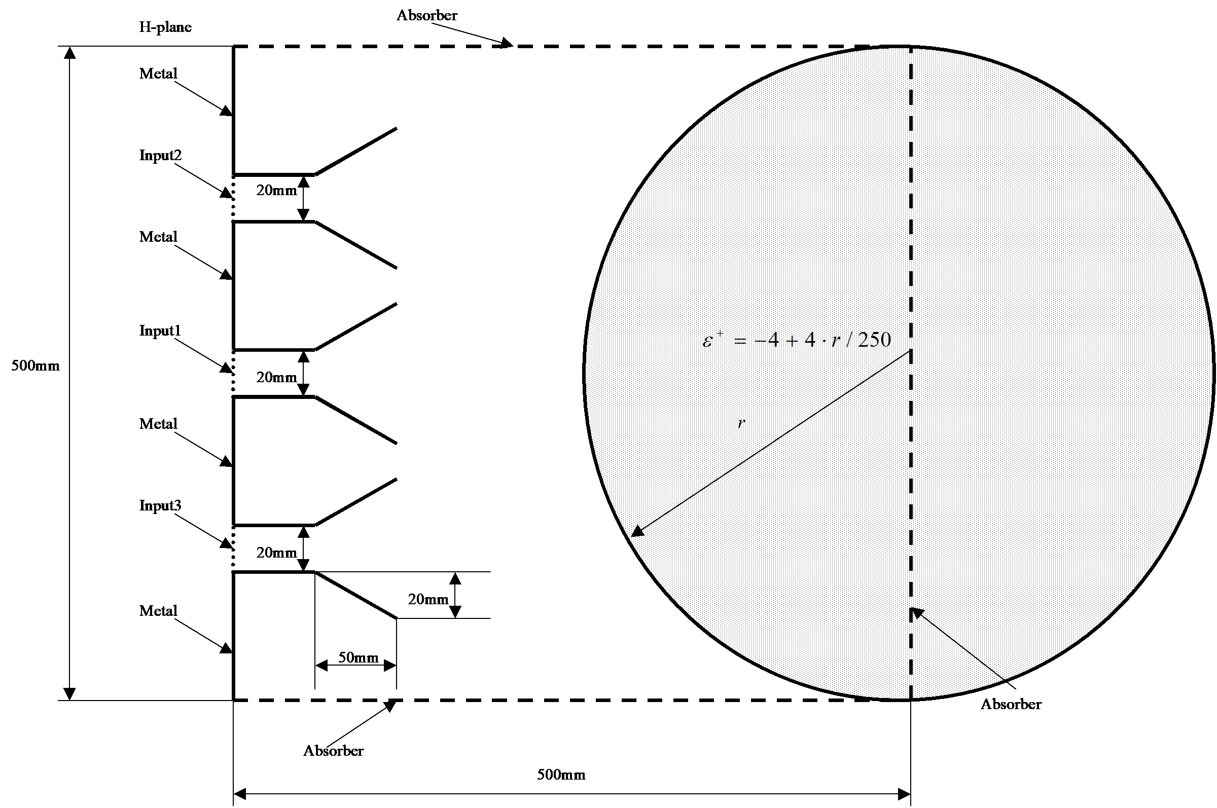
Рис. 6.1. Система из трёх рупоров для изучения рассеяния на неоднородном диэлектрическом цилиндре радиусом 250 мм. Проницаемость цилиндра зависит от радиуса: на границе равна 1, в центре −5.
Центральный рупор излучает сигнал, два боковых — приёмные.
Ключевые места задания:
#define W_eps @ ( -4 + 4*r/(W_waveg/2)+1 )
…
 BLOCK 104;
  CIRCLE_STAT (W_eps-1); 0; W_waveg/2; 0; 2*3.1415;
 END_B
…
 BLOCK 8;
  RECT_STAT ABSORBER; L_waveg-5*W_delta; L_waveg - 1*W_delta+0.00; 0.0; W_waveg-2*W_delta;
 END_B
Здесь:
W_eps— функция от полярного радиусаr: на границе (r = W_waveg/2) даёт 1, в центре (r = 0) даёт −4 + 1 = −3;- в блок передаётся
(W_eps-1)— снова добавка; - блоки 8, 9, 10 — поглотители по краям коробки, чтобы волна не отражалась от стенок. Обратите
внимание, как их границы отступают от границ коробки на несколько
W_delta— это выполнение требования из раздела 5.2; - рупоры собраны из
RECT_STAT METAL(стенки) иPOLYGON_STAT METAL(раскрывы), причём одна и та же группа блоков повторена трижды с разными номерами и размещена в#LINK_LISTна разных высотах (W_waveg/2,W_waveg/4,3*W_waveg/4).
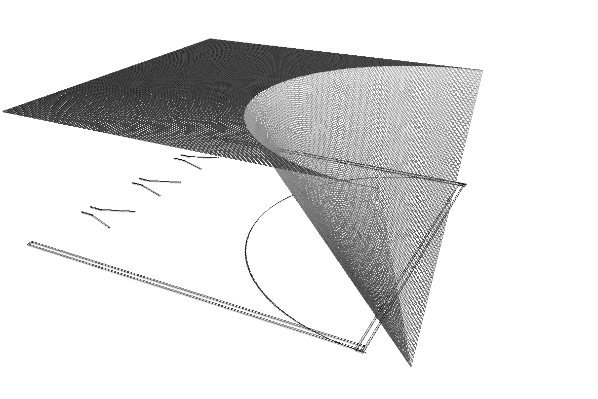
Рис. 6.2. Распределение диэлектрической проницаемости, как его показывает FieldView.
12. Таблица ключевых слов
Обозначения: expression — математическое выражение; expression(x,y,r,f) — выражение от
декартовых или полярных координат; n — целое число; < > — обязательный параметр; [ ] —
необязательный.
| Ключевое слово | Формат | Назначение |
|---|---|---|
#TMC_RT_H |
Начало файла задания | |
#STEP |
Начало шага задания | |
#PARM |
Начало секции параметров | |
ANGLE_UNIT |
<radian> \| <gradus>; |
Единицы измерения углов |
FREQ_UNIT |
<GHz> \| <MHz> \| <kHz> \| <Hz>; |
Единицы измерения частоты |
LONG_UNIT |
<mm> \| <cm> \| <m>; |
Единицы измерения длины |
TIME_UNIT |
<s> \| <ms> \| <mks> \| <ns> \| <ps>; |
Единицы измерения времени |
DELTA |
<expression>; |
Точность анализа — размер пространственного дискрета |
TIME |
<expression>; <expression>; |
Время анализа T_min; T_max |
X_MIN |
<expression>; |
Абсцисса левого края «коробки» |
X_MAX |
<expression>; |
Абсцисса правого края «коробки» |
Y_MIN |
<expression>; |
Ордината нижнего края «коробки» |
Y_MAX |
<expression>; |
Ордината верхнего края «коробки» |
FREQ |
<expression>; |
Частота сигналов возбуждения |
HEIGHT |
<expression>; |
Разбирается, на расчёт не влияет (раздел 4.9) |
DELTA_T_MECHANICAL |
<expression>; |
Разбирается, на расчёт не влияет (раздел 4.9) |
N_UNIT |
<m3> \| <cm3> \| <mm3>; |
Разбирается, множитель не применяется (раздел 4.9) |
B_UNIT |
<Tl> \| <mTl> \| <mkTl>; |
Разбирается, множитель не применяется (раздел 4.9) |
#END_PARM |
Конец секции параметров | |
#TOPOLOGY |
Начало секции геометрии | |
BLOCK |
<n>; |
Начало блока, n > 0 |
RECT_STAT |
[[file_name]]<METAL> \| <MAGNETIC> \| <ABSORBER> \| <expression(x,y,r,f)>; <X_min>; <X_max>; <Y_min>; <Y_max>; |
Неподвижный прямоугольник |
CIRCLE_STAT |
<METAL> \| <MAGNETIC> \| <ABSORBER> \| <expression(x,y,r,f)>; <R_min>; <R_max>; <F_min>; <F_max>; |
Неподвижный сектор |
POLYGON_STAT |
<METAL> \| <MAGNETIC> \| <ABSORBER> \| <expression(x,y,r,f)>; |
Неподвижный многоугольник |
L |
<expression>; <expression>; |
Точка многоугольника X0; Y0; |
INPUT_X |
[<METAL> \| <MAGNETIC>]; <Y_min>; <Y_max>; <T_min>; <T_max>; [<Amp>]; [<Faza>]; [<Eps>]; |
Вход вдоль оси Y (на левой/правой границе) |
INPUT_Y |
[<METAL> \| <MAGNETIC>]; <X_min>; <X_max>; <T_min>; <T_max>; [<Amp>]; [<Faza>]; [<Eps>]; |
Вход вдоль оси X (на нижней/верхней границе) |
FILE |
<file_name>; <X_min>; <X_max>; <Y_min>; <Y_max>; |
Чтение распределения ε из файла |
RECT_STAT_N, CIRCLE_STAT_N, POLYGON_STAT_N, FILE_N |
как у базового примитива | Концентрация плазмы N, м⁻³ (X-мода) |
RECT_STAT_B, CIRCLE_STAT_B, POLYGON_STAT_B, FILE_B |
как у базового примитива | Индукция B, Тесла (X-мода) |
RECT_STAT_Y, CIRCLE_STAT_Y, POLYGON_STAT_Y, FILE_Y |
как у базового примитива | Параметр Y (X-мода) |
RECT_MOVE, CIRCLE_MOVE, POLYGON_MOVE |
не документировано | Подвижные блоки |
END_B |
Конец блока | |
#END_TOPOLOGY |
Конец секции геометрии | |
#LINK_LIST |
Начало секции графа связей | |
T |
<n>; <expression>; <expression>; |
Поместить начало координат блока n в точку X0; Y0; |
#END_LINK |
Конец секции графа связей | |
#OUTPUT |
Начало секции выходных данных | |
FILE |
<file_name>; |
Сигналы на входах → file_name.t (обязательно, первым) |
TOPOLOGY |
Вывод топологии → file_name.tt |
|
FIELDS |
Вывод распределения полей | |
SMATRIX |
<Sfile>; <expression>; <T_min>; <T_max>; |
S-матрица → Sfile.s |
FIELD_DISTRIBUTION |
<file_name>; <freq>; <expression>; <expression>; |
Комплексное распределение поля |
FIELD_DISTRIBUTION_M |
<file_name>; <freq>; <expression>; <expression>; |
То же, с накоплением в памяти |
#END_OUTPUT |
Конец секции выходных данных | |
#END_STEP |
Конец шага задания | |
#EOF |
Конец входного задания | |
#define |
<имя> [par1; …] @ <текст> |
Макроопределение (препроцессор) |
#include |
<file_name> |
Вставка файла (препроцессор) |
! |
Комментарий (до конца строки) |
13. Типичные ошибки
| Симптом | Причина |
|---|---|
| Ширина/длина блока «не та» | Макрос без скобок: #define L @ 38+12 вместо #define L @ (38+12). См. 9.2 |
Ошибка «Missing file name» / Unresolved simbol '.' |
Имя в FILE пустое или содержит точку. См. 7.1 |
Пустой .s, «Error when read» в TMCGROUT |
SMATRIX задан на одной частоте (одна точка — кривая не строится) либо окно T_min…T_max вне интервала сигнала. См. 7.4 |
| FieldView ничего не показывает | Включён FIELDS, но не включён TOPOLOGY. См. 7.2 |
| Расчёт идёт очень долго | Слишком мелкий DELTA (время растёт как куб) либо включён FIELDS при свипе. См. 4.5, 10 |
Неверный результат у POLYGON_STAT с ε |
Область незамкнута, невыпукла или вершины обойдены против часовой стрелки — не диагностируется. См. 5.4 |
| Частотная характеристика сдвинута относительно аналитики | Свойство метода (длина волны в сетке). Погрешность выводится в окне статистики. См. 10 |
| Блок не появился в расчёте | Для блока нет строки T в #LINK_LIST. См. 6 |
CIRCLE_STAT_B ведёт себя как CIRCLE_STAT_N |
Известный дефект диспетчера, не исправлен. См. 5.7 |
14. Источники
Документ восстановлен по авторским материалам из архива I:\Python Project\Tamic\data Tamic\
и сверен с исходным кодом TMC Suite.
Использовано:
| Документ | Что взято |
|---|---|
TMC\DISTR\MANUALS\RT_HPLANAR\rt_hplanar.doc (2.6 МБ, 2000) |
Основной источник. Полное описание входного языка, методика составления задания, все рисунки примитивов, примеры |
TMC\DISTR\MANUALS\RT_HPLANAR\FormEps.doc (1999) |
Формат распределения ε |
TMC\DISTR\TMC_I\TMC\DOC_SRC\S_FILE.DOC (1992) |
Формат S-файла (см. docs/api/libs/sfile95.md) |
Рисунки извлечены из rt_hplanar.doc (векторные WMF → PNG) и лежат в docs/screenshots/tpl/.
Проверено и отклонено как не относящееся к TMC Suite:
| Документ | Почему не подошёл |
|---|---|
TMC\DISTR\MANUALS\TAMICE_H.DOC (898 КБ, 1999) |
Отчёт о НИР по родственному продукту TAMIC-E/H. Другой входной язык: #PARMS, FRQS, TOLERANCE, WIDTH, GRAPH_K. Полезен как объяснение разнобоя #PARM/#PARMS (раздел 4) |
TMC\DISTR\EMSTAR\MANUAL.DOC |
Продукт EMSTAR — планарный ЭМ-симулятор со своим языком (LAYER, MEDIA, PORT, EMFRQS). К TMC Rt отношения не имеет |
TMC\DISTR\MANUALS\{E2R,H2R,I1R,I2E,I2R,M2E,M2R,W2R}\*.DOC |
Руководства других анализаторов семейства TAMIC |
15. Связанные документы
docs/user-manual/planar_rt_h.md— руководство пользователя ядра Hdocs/user-manual/planar_rt_x.md— руководство пользователя ядра Xdocs/user-manual/fieldview.md— просмотр полей и топологииdocs/user-manual/tmcros.md— просмотр сигналов.tdocs/user-manual/tmcgrout.md— просмотр S-матриц.sdocs/api/libs/prepr.md— API препроцессораdocs/api/libs/tmcindan.md— API разбора входного языкаISSUES.md— известные дефекты
The .tpl template file — how to create it. A complete reference of the input language
Applies to the compute kernels PlanarRT_H (
tmc_rth.exe) and PlanarRT_X (tmc_rtx.exe).The document has been reconstructed from the author's manual "TAMIC-Rt H. A program for the electrodynamic analysis of planar structures with inhomogeneous dielectric filling in the H-plane, version 2.0p" (TAMIC_soft group, 2000) and checked against the current source code of TMC Suite. Places where the current code diverges from the 2000 manual are marked explicitly — in case of a discrepancy, the code is considered correct.
1. What the template file is
The input data of a compute kernel is the geometry of the device under analysis, which is
described in a text template file with the .tpl extension. The kernel reads the .tpl, performs
the computation and produces results as files of several types, which are then viewed with the
package's viewers.
Block diagram of the package (fig. 2.1 of the author's manual).
Discrepancy with the figure. In the 2000 diagram the field file is labelled
File.ft, while the text of the same manual calls itFile.tf. In the current code the field is written to the files.ex/.ey/.hz/.em/.ef(see section 8). The.tfextension survives only in the list of formats FieldView can open.
This separation (computing on one side, viewing on the other) makes the system more flexible and minimises the computer resources required to run a computation.
2. General structure of the template file
Every line of the file starts with a unique descriptor that defines the data following it.
The template file always begins with the line #TMC_RT_H and ends with the line #EOF.
The whole template is divided into steps. Each step may describe an independent microwave device
or a part of one; a step begins with the line #STEP and ends with #END_STEP:
#TMC_RT_H          Start of the template file
#STEP              This is the first step
   Data for the first problem
#END_STEP
#STEP              This is the second step
   Data for the second problem
#END_STEP
#EOF               End of the template file
The
#TMC_RT_Hsignature is common to both kernels. The X-kernel (tmc_rtx.exe) reads files with the same first line#TMC_RT_H; there is no separate#TMC_RT_Xsignature in the code.
Each step consists of four sections, which are best placed in this order:
| Section | Purpose | Required? |
|---|---|---|
#PARM … #END_PARM |
Units, grid step, time, box boundaries, frequency | In the first step — yes |
#TOPOLOGY … #END_TOPOLOGY |
The blocks (graphic primitives) the device is made of | Yes |
#LINK_LIST … #END_LINK |
The geometric position of each block inside the box | Yes |
#OUTPUT … #END_OUTPUT |
Which output files to produce | Yes (at least FILE is needed) |
The parameter section may be omitted in the steps that follow the first one — then the parameters are taken to be the same as in the previous step.
2.1. Syntax
- All operators carrying the
#symbol must start at the first position of the line. - The other operators must have at least one space in the first position of the line.
- A comment is any line, or part of a line, starting with the
!symbol. - Empty lines and lines of spaces only are allowed.
- Parameters are separated from the line identifier by at least one space, and from each other by
the
;symbol.
The formalised format notations below use the following conventions:
| Notation | Meaning |
|---|---|
< > |
a required parameter |
[ ] |
an optional parameter |
expression |
a mathematical expression |
expression(x,y,r,f) |
an expression containing a function of Cartesian (x, y) or polar (r, f) coordinates |
n |
an integer |
3. Method: how to write a template from scratch
This is the very order of actions the author used. Let us go through it on the problem from the author's manual: the scattering of a plane wave on a plane-parallel plate with ε = 4 at a frequency of 10 GHz.
Step 1. Draw the topology in the H-plane
You start with a drawing of the real device in the H-plane, with all its dimensions.
The placement of the plane-parallel plate in the H-plane (fig. 3.1). All dimensions are in millimetres.
Step 2. Fit the device into a "box"
The whole device must fit inside a rectangle — it is called the "box". The position of the box is
given in the parameter section by the values X_MIN, X_MAX, Y_MIN, Y_MAX.
The boundary of the box is metal or the inputs of the device. This matters: the box boundary itself is always metal, unless an input stands on it.
The placement of the plate inside the "box" and the values of the constant expressions to be set (fig. 3.2).
Note the notation ε⁺ = 3 inside the plate: this is not the permittivity itself but the increment over the permittivity of vacuum. A plate with ε = 4 corresponds to an increment of ε⁺ = 3 (see section 5.1).
Step 3. Decompose the geometry into primitives
The resulting geometry is decomposed into blocks — the graphic primitives of the input language.
The decomposition of the given geometry using graphic primitives (fig. 3.3).
For our problem this gives five blocks:
| Block | What it is |
|---|---|
| Block 1, Block 2 | the inputs of the device (INPUT_X) |
| Block 3, Block 4 | rectangles with magnetic walls (RECT_STAT MAGNETIC) |
| Block 5 | a rectangle with a given dielectric distribution (RECT_STAT) |
Step 4. Choose the grid step Δ
The grid step DELTA determines the accuracy. The rules for choosing it are in section 4.5. In
short: roughly 1/20 of the wavelength in the waveguide at the maximum frequency of the range
gives an accuracy of about 3 %.
Step 5. Write the template
Each block is described in the #TOPOLOGY section in its own local coordinate system, and is
then placed inside the box by a T line in the #LINK_LIST section.
The full text of the template (the file samples/SAMPLE_R/TEST_MAG/EPS4/TEST0.TPL, quoted after the
author's manual — the file in the repository has been changed since, see the note below):
#TMC_RT_H
#define L1 @ (   50.00)
#define L2 @ (   50.00)
#define L3 @ (   50.00)
#define W_freq @ (  10 )
#define W_eps @ ( 4.00 )
#define W_waveg @ (  6.00 )
#define W_input @ (  2.00 )
#define W_delta @ (    0.5 )
#define W_type @ MAGNETIC
#define a1 @ ( W_input )
#STEP
#PARM
 ANGLE_UNIT radian;
 FREQ_UNIT GHz;
 LONG_UNIT mm;
 TIME_UNIT ns;
 DELTA W_delta;
 TIME 0.; 5;
 X_MIN  0.0;
 X_MAX L1+L2+L3;
 Y_MIN  0.0;
 Y_MAX W_waveg;
 FREQ  10;
#END_PARM
#TOPOLOGY
 BLOCK 1;
  INPUT_X   W_type ; -a1/2; a1/2; 0; 200;
 END_B
 BLOCK 2;
  INPUT_X    W_type ; -a1/2; a1/2; 200; 201;
 END_B
 BLOCK 3;
  RECT_STAT W_type ; 0.0; L1+L2+L3; -a1/2-2*W_delta; -a1/2-1*W_delta;
 END_B
 BLOCK 4;
  RECT_STAT W_type ; 0.0;L1+L2+L3; a1/2; a1/2+W_delta;
 END_B
 BLOCK 5;
  RECT_STAT (W_eps-1); 0;L2; 0.0; W_waveg;
 END_B
#END_TOPOLOGY
#LINK_LIST
 T 1; 0.0; W_waveg/2;
 T 2; L1+L2+L3; W_waveg/2;
 T 3; 0.0; W_waveg/2;
 T 4; 0.0; W_waveg/2;
 T 5; L1; 0.0;
#END_LINK
#OUTPUT
 FILE test1;
 SMATRIX test1; 10; 4; 5;
 FIELDS;
 TOPOLOGY;
#END_OUTPUT
#END_STEP
#EOF
A walk-through of the key places:
#define W_eps @ ( 4.00 )— the permittivity of the plate, ε = 4;RECT_STAT (W_eps-1); …— the block is passed the increment ε⁺ = ε − 1 = 3. Hence the-1;INPUT_X W_type; -a1/2; a1/2; 0; 200;— an input of widtha1, an RF pulse from 0 to 200 ns;- the second input (Block 2) has
T_min = 200, which is greater than the analysis time (TIME 0.; 5;) — this is how you define an input that has no incident wave, only reception; SMATRIX test1; 10; 4; 5;— write the S-matrix for the frequency of 10 GHz, averaged from 4 to 5 ns.
The file in the repository differs from the manual. In
samples/SAMPLE_R/TEST_MAG/EPS4/TEST0.TPLthe valuesL1=100,L2=600,L3=100,W_eps=-0.01,W_delta=0.1,TIME 0.; 200;have been changed since 2000, and the first input has gained extra parameters (… 0; 200; 1.; ;— amplitude and phase, see section 6.4). The text above is the one from the manual; it shows the original intent.
Step 6. Check and run
- Open the
.tplin the kernel (File → Open). - Parsing errors are reported with the line number — the language is checked strictly.
- Run the computation and look at the results with the viewers (section 8).
4. The parameter section #PARM
#PARM
    . . .
#END_PARM
#PARMor#PARMS? In the author's manual of 2000 the "Input format" parts of items 4.1.x are written with#PARMS/#END_PARMS(11 places), while all the real examples and the table of contents use#PARM/#END_PARM. This is a trace of the related product TAMIC-E/H, where the section really is called#PARMS.Both variants work. The canonical names in the code are
#PARMand#END_PARM(src/Include/TmcRTH_Indan.h, line 23), but sections are searched for by comparing prefixes (strncmp(csCh, csSection, csSection.GetLength())inTmcRTH_Indan.cpp, lines 435 and 460), so#PARMSand#END_PARMSmatch as well. Writing#PARM/#END_PARMis recommended.
The units of angle, frequency, length and time must be set before the frequencies and the parameters that have the dimension of length and time are defined.
The section must be present in the first step. If it is absent in the other steps, the parameters are the same as in the previous step.
4.1. ANGLE_UNIT — the unit of angle
ANGLE_UNIT <radian> | <gradus>;
Fixes the unit of the angle arguments of trigonometric functions.
| Value | Meaning |
|---|---|
radian |
radians |
gradus |
degrees |
The default is the same as in the previous step; if this is the first step — radian.
4.2. FREQ_UNIT — the unit of frequency
FREQ_UNIT <GHz> | <MHz> | <kHz> | <Hz>;
Entered before the FREQ line. The default in the first step is GHz.
4.3. LONG_UNIT — the unit of length
LONG_UNIT <mm> | <cm> | <m>;
Entered before the DELTA, X_MIN, X_MAX, Y_MIN, Y_MAX lines. The default in the first
step is mm.
4.4. TIME_UNIT — the unit of time
TIME_UNIT <s> | <ms> | <mks> | <ns> | <ps>;
Entered before the TIME line.
According to the author's manual, the default value in the first step is seconds (
s), notns. It is better to set the time unit explicitly.
4.5. DELTA — the grid step (accuracy of the analysis)
DELTA <expression>;
Its physical meaning is the size of the spatial sample, the step of the square grid the whole device is split into. This is the main accuracy parameter.
The author's recommendations:
- For an accuracy of about 3 % the value should be about 1/20 of the wavelength in the waveguide at the maximum frequency of the range. More precisely — it is determined by a series of convergence computations.
- As the step decreases, the analysis time grows as its cube. For this reason the initial work on a device is done at low accuracy, which is raised at the final stage.
- Choose the step and the geometry so that the geometry fits a whole number of samples. If the
metal thickness is 1, 2, 3, 4 mm — take
DELTA= 1 mm or 0.5 mm, not 1.02 mm or 0.47 mm. - The computation time is at its minimum when a whole number of samples fits into the "box" along X and Y.
The parameter is required in the first step.
4.6. TIME — the analysis time
TIME <expression>; <expression>;
The first parameter is the start time of the analysis, the second is the end time. Required in the first step.
4.7. X_MIN, X_MAX, Y_MIN, Y_MAX — the boundaries of the "box"
X_MIN <expression>;
X_MAX <expression>;
Y_MIN <expression>;
Y_MAX <expression>;
They define the rectangle the topology under analysis is placed into. Required in the first step.
4.8. FREQ — the frequency of the excitation signals
FREQ <expression>;
The frequency of the excitation signals at the inputs of the device. Required in the first step.
4.9. Parameters accepted by the code but not affecting the computation
These lines are parsed and their values stored, but no kernel reads them. Verified against the
sources: the corresponding getters (dGetHeight, GetDeltaT, IsDeltaTDefine) are not called from
kernels/, from fieldview/ or from viewers/; the rNUnit / rBUnit fields are not read outside
the parsing module.
| Keyword | Format | State |
|---|---|---|
HEIGHT |
HEIGHT <expression>; |
Parsed, does not affect the computation. Occurs in samples/SAMPLE_R/TEST_*/…/HWVGD_1.TPL (HEIGHT 0.1;) |
DELTA_T_MECHANICAL |
DELTA_T_MECHANICAL <expression>; |
Parsed, calls SetDeltaT(), but the result is not read |
N_UNIT |
N_UNIT <m3> \| <cm3> \| <mm3>; |
Parsed, the multiplier is not applied |
B_UNIT |
B_UNIT <Tl> \| <mTl> \| <mkTl>; |
Parsed, the multiplier is not applied |
Practical consequence: the plasma concentration N in *_STAT_N blocks is always treated as
m⁻³, and the induction B in *_STAT_B blocks is always in Tesla, regardless of what is
written in N_UNIT / B_UNIT.
To be clarified with the author (K. N. Klimov): were
HEIGHTandDELTA_T_MECHANICALmeant to be working parameters? At present they are not connected to the computation.Defect (a candidate for
ISSUES.md): theReadNUnitfunction insrc/libs/TMCIndan/TmcRTH_IndanParam.cpp(lines ~1211–1224) writes its result into thecsBUnit/rBUnitfields instead ofcsNUnit/rNUnit— an obvious copy-paste error. It is harmless at present (neither field is used), but it will become a bug if the units are connected to the computation. Besides, theN_UNITmultipliers raise a question:cm3 → 0.000001, whereas 1 cm⁻³ = 10⁶ m⁻³.
5. The topology section #TOPOLOGY
#TOPOLOGY
    BLOCK 1;
        <the primitive type and its parameters>
    END_B
    . . .
    BLOCK <n>;
        . . .
    END_B
#END_TOPOLOGY
Every block is given a unique number <n> — an integer greater than zero. The numbers do not
have to be in order and do not have to be contiguous (the author's example with horns uses the
numbers 1, 2, 5, 6, 7, 12, 14, 21, 22, 25, 26, 41…46, 104).
The parameters of every primitive are described in its own local coordinate system. The position
of a block inside the box is defined in #LINK_LIST — therefore every block must have exactly one
matching line in #LINK_LIST.
All primitives except the inputs (INPUT_X, INPUT_Y) may overlap and intersect each other. The
inputs must be placed only on the boundary of the "box".
5.1. The material or the ε distribution
The first parameter of a primitive defines either the material or the distribution of the permittivity increment:
| Value | Meaning |
|---|---|
METAL |
metal (a perfect conductor) |
MAGNETIC |
a magnetic — an open-circuit wall (a magnetic wall) |
ABSORBER |
an absorber |
expression(x,y,r,f) |
the distribution of the increment ε⁺ over the permittivity of vacuum |
The key convention: it is the increment that is given, not the permittivity itself.
| The ε you need | What to write |
|---|---|
| ε = 4 | 3 |
| ε = 9 | 8 |
| ε = 1 (vacuum) | 0 |
| ε = 0 | -1 |
| ε = 0.25 | -0.75 |
An important difference in the meaning of a primitive — a material defines the CONTOUR, not the fill. If a material is given, the primitive defines a boundary (a contour, a polyline). If an expression is given, the primitive defines an area filled with a medium. This is clearly visible in the figures below: with
RECT_STAT METALonly the contour of the rectangle is metal, while withRECT_STAT 8the whole area is filled.Confirmed by the code:
SetRectMetal(src/kernels/PlanarRT_H/TmcRTHNodeDiel.cpp:2419) allocatesnNumNode = 2*nX + 2*(nY-1)nodes — this is the perimeter, notnX*nY(a fill) — and fills them in four loops: the bottom edge (y = dYmin), the top one (y = dYmax), the left one (x = dXmin) and the right one (x = dXmax).Practical consequence. To get a solid metal object, define it by its contour: the field does not penetrate inside a closed contour. And to get a solid dielectric insert — give an expression, it fills the area.
Careful,
METALandMAGNETICswap places. Insrc/Include/Tmcgrviw.h(lines 159–165) the definitions depend on the_MODEL_RTE__macro: when it is present,METALandMAGNETICswap roles (the E-plane model). In the regular H and X builds this macro is not defined, and the words mean what they say.
5.2. RECT_STAT — a fixed rectangle
BLOCK <n>;
    RECT_STAT [[file_name]]<METAL> | <MAGNETIC> | <ABSORBER> | <expression(x,y,r,f)>;
    <X_min>; <X_max>;
    <Y_min>; <Y_max>;
END_B
| № | Parameter | Meaning |
|---|---|---|
| 1 | material / expression | see section 5.1 |
| 2 | X_min |
the left boundary along X |
| 3 | X_max |
the right boundary along X |
| 4 | Y_min |
the lower boundary along Y |
| 5 | Y_max |
the upper boundary along Y |
The optional [file_name] in square brackets before the expression means save the computed ε
distribution into the file file_name.eps, so that it can later be reused by the FILE primitive
(section 5.6). It is needed to improve efficiency when computations over large areas are repeated.
Two additional conditions for MAGNETIC and ABSORBER:
- The differences
X_max − X_minandY_max − Y_minmust exceed2*DELTA— the thickness and the height must be greater than two spatial samples. - The whole rectangle must be inside the box, and its boundary must be at least one grid step away from the boundary of the box.
Examples
Fig. 4.1. A fixed rectangle of 30×10 mm bounded by metal.
BLOCK 1;
    RECT_STAT METAL; 0; 30; 0; 10;
END_B
Fig. 4.2. A rectangle of 29×8 mm with open-circuit walls (a magnetic).
BLOCK 1;
    RECT_STAT MAGNETIC; -29; 0; -8; 0;
END_B
Fig. 4.3. A rectangle of 27×9 mm with absorbing walls.
BLOCK 1;
    RECT_STAT ABSORBER; 0; 27; 0; 9;
END_B
Fig. 4.4. A rectangle of 31×12 mm with ε = 4 (the increment ε⁺ = 3).
BLOCK 1;
    RECT_STAT 3; 0; 31; 0; 12;
END_B
Fig. 4.5. A rectangle of 31×12 mm with ε = 0 (the increment ε⁺ = −1).
BLOCK 1;
    RECT_STAT -1; 0; 31; 0; 12;
END_B
Fig. 4.6. A rectangle of 30×10 mm; ε falls linearly along X from 1 at the left boundary to −1 at the right one (the increment changes from 0 to −2).
BLOCK 1;
    RECT_STAT -2*x/30; 0; 30; 0; 10;
END_B
5.3. CIRCLE_STAT — a fixed sector
BLOCK <n>;
    CIRCLE_STAT <METAL> | <MAGNETIC> | <ABSORBER> | <expression(x,y,r,f)>;
    <R_min>; <R_max>;
    <F_min>; <F_max>;
END_B
| № | Parameter | Constraint |
|---|---|---|
| 1 | material / expression | see section 5.1 |
| 2 | R_min |
≥ 0 |
| 3 | R_max |
> R_min |
| 4 | F_min |
≥ 0 |
| 5 | F_max |
> F_min, ≤ 2π |
R_min, R_max are in LONG_UNIT units; F_min, F_max are in ANGLE_UNIT units.
Examples
Fig. 4.7. A metal circle with a radius of 30 mm.
BLOCK 1;
    CIRCLE_STAT METAL; 0; 30; 0; 2*3.141592653589;
END_B
Fig. 4.8. A semicircle made of a magnetic with a radius of 29 mm.
BLOCK 1;
    CIRCLE_STAT MAGNETIC; 28.9; 29; 3.141592653589/2; 3*3.141592653589/2;
END_B
Fig. 4.9. A half-disc made of an absorber with a radius of 27 mm.
BLOCK 1;
    CIRCLE_STAT ABSORBER; 0; 27; 0; 3.141592653589;
END_B
Fig. 4.10. A circle with a radius of 30 mm and ε = 9 (the increment ε⁺ = 8).
BLOCK 1;
    CIRCLE_STAT 8; 0; 30; 0; 2*3.141592653589;
END_B
Fig. 4.11. A sector with ε = −1 (the increment ε⁺ = −2).
BLOCK 1;
    CIRCLE_STAT -2; 10; 30; 3.141592653589/2; 3.141592653589;
END_B
5.4. POLYGON_STAT — a fixed polygon
BLOCK <n>;
    POLYGON_STAT <METAL> | <MAGNETIC> | <ABSORBER> | <expression(x,y,r,f)>;
        L <expression>; <expression>;
        L <expression>; <expression>;
        L <expression>; <expression>;
        [L <expression>; <expression>;]
        …
END_B
The first line carries the material or the expression. In the following lines, after the L symbol,
the abscissa and the ordinate of a vertex are entered in the local coordinate system of the block.
The behaviour depends on the first parameter — this matters:
| First parameter | Behaviour |
|---|---|
| an expression (ε) | The last point is connected to the first one, forming a closed area. The area must be simply connected and convex, and the vertices must be traversed clockwise. The number of vertices must be greater than 3. |
METAL, MAGNETIC, ABSORBER |
The last point is not connected to the first one — a polyline is formed rather than a closed area. The traversal direction and convexity need not be respected. |
The program does not check whether the area is closed and simply connected, nor whether the vertices are traversed in the right direction. An error here is not diagnosed — it will show up as a wrong result.
Examples
Fig. 4.12. A metal quadrangle (closed explicitly — the first point is repeated at the end).
BLOCK 1;
    POLYGON_STAT METAL;
        L -10; 0;
        L 0; 10;
        L 10; 0;
        L 0; -10;
        L -10; 0;
END_B
Fig. 4.13. A metal polyline (the same text without repeating the first point).
BLOCK 1;
    POLYGON_STAT METAL;
        L -10; 0;
        L 0; 10;
        L 10; 0;
        L 0; -10;
END_B
Fig. 4.14. A dielectric quadrangle with ε = 4 (the increment ε⁺ = 3) — the area closes itself.
BLOCK 1;
    POLYGON_STAT 3;
        L -10; 0;
        L 0; 10;
        L 10; 0;
        L 0; -10;
END_B
Fig. 4.15. A polyline made of a magnetic wall.
BLOCK 1;
    POLYGON_STAT MAGNETIC;
        L -10; 0;
        L 0; 10;
        L 10; 0;
END_B
Fig. 4.16. A polyline made of an absorber.
BLOCK 1;
    POLYGON_STAT ABSORBER;
        L 10; 0;
        L 0; -10;
        L -10; 0;
END_B
Fig. 4.17. A dielectric triangle with ε = 0.25 (the increment ε⁺ = −0.75).
BLOCK 1;
    POLYGON_STAT -0.75;
        L 10; 0;
        L 0; -10;
        L -10; 0;
END_B
5.5. INPUT_X and INPUT_Y — the inputs (excitation transformers)
By their functional purpose the blocks fall into two types: excitation transformers and internal areas. All the primitives above are internal areas.
Careful with the names — they do not mean what they seem to.
INPUT_Xis an input along the Y axis; it is placed on the left or right boundary of the box, and its dimensions are given along Y.INPUT_Yis an input along the X axis; it is placed on the bottom or top boundary of the box, and its dimensions are given along X. Which boundary an input actually ends up on is determined by the coordinates in#LINK_LIST.
BLOCK <n>;
    INPUT_X [<METAL> | <MAGNETIC>];
    <Y_min>; <Y_max>;
    <T_min>; <T_max>;
    [<Amplitude>]; [<Faza>];
    [<Eps>];
END_B
BLOCK <n>;
    INPUT_Y [<METAL> | <MAGNETIC>];
    <X_min>; <X_max>;
    <T_min>; <T_max>;
    [<Amplitude>]; [<Faza>];
    [<Eps>];
END_B
Parameters 1–5 (documented in the 2000 manual):
| № | Parameter | Meaning |
|---|---|---|
| 1 | type | The mode of the incident wave (see the table below) |
| 2 | Y_min / X_min |
The lower (left) boundary of the input |
| 3 | Y_max / X_max |
The upper (right) boundary of the input, > min |
| 4 | T_min |
The start time of the excitation RF pulse |
| 5 | T_max |
The end time of the excitation RF pulse, > T_min |
The excitation mode is given by the first parameter:
| Value | Mode | Requirement on the input width |
|---|---|---|
MAGNETIC |
a plane wave | the width is less than half the wavelength of the input signal |
METAL or empty |
the first oscillation type of a rectangular waveguide (the H₁₀ wave) | the width is greater than half but less than the full wavelength |
These conditions must be met so that a single-mode regime of excitation and matching is realised in the input cross-section. The mode the reflected signal is observed in matches the incident one.
The frequency of the RF pulse is set by the FREQ parameter from the parameter section.
How to define an input with no incident wave (receive-only). If there is no incident wave at an input,
T_minmust be greater than the analysis time from the parameter section (TIME). This is exactly how the second input in the example of section 3 is made:TIME 0.; 5;withINPUT_X …; 200; 201;.
Parameters 6–8 are an extension that is not in the 2000 manual.
Established from the source code (ReadInputX / ReadInputY in
src/libs/TMCIndan/TmcRTH_BolckList.cpp; the computation — dAmplitude, dFaza,
CalculateYForInput in src/kernels/PlanarRT_H/TmcRTHNodeDiel.cpp):
| № | Parameter | Meaning | If not given |
|---|---|---|---|
| 6 | Amplitude |
The amplitude of the signal — an expression in the variables t (the current time) and f (the frequency) |
1.0 |
| 7 | Faza |
The phase of the signal — an expression in t and f, in ANGLE_UNIT units |
0.0 |
| 8 | Eps |
The ε increment in the cross-section of the input (affects the wave conductance of the input) | not applied |
All three are optional, but parameter 7 is required if parameter 6 is given (otherwise you get the
error "Missing separator ';'"). An empty value is allowed: … 0; 200; 1.; ; means an amplitude of 1.0
and the default phase — this is exactly how the first input is written in the current
samples/SAMPLE_R/TEST_MAG/EPS4/TEST0.TPL.
The variables t and f make it possible to define the envelope of the pulse instead of a
rectangular RF pulse — a Gaussian one, for example.
The code fields that hold these parameters (
csVx,csVy,csW) mean something entirely different for moving blocks (RECT_MOVEand the like) — the linear and angular velocities. The comment insrc/Include/TmcRTH_BolckList.h(lines 139–141) records both meanings.To be clarified with the author (K. N. Klimov): parameter 8 (
Eps) — is it the ε⁺ increment or ε itself that is given? The check in the code reads(r + 1.0) <= 0.0, which corresponds to the increment (ε = r + 1 > 0).
Examples
Fig. 4.18. A waveguide input (H₁₀) 20 mm wide; it excites the system with an RF pulse 10 ns long.
BLOCK 1;
    INPUT_X METAL; 0; 20; 0; 10;
END_B
Fig. 4.19. An input for a plane wave 2 mm wide, an RF pulse 100 ns long.
BLOCK 1;
    INPUT_X MAGNETIC; 0; 2; 0; 100;
END_B
Fig. 4.20. A waveguide input (H₁₀) 20 mm wide along the X axis. The type is not given — the
equivalent of METAL.
BLOCK 1;
    INPUT_Y ; 0; 20; 0; 10;
END_B
Fig. 4.21. An input for a plane wave 2 mm wide along the X axis.
BLOCK 1;
    INPUT_Y MAGNETIC; 0; 2; 0; 100;
END_B
5.6. FILE — reading an ε distribution from a file
BLOCK <n>;
    FILE <file_name>;
    <X_min>; <X_max>;
    <Y_min>; <Y_max>;
END_B
When the ε distribution is computed for large areas of rectangles, evaluating the formula at every
node takes a noticeable amount of time. It can be done once, saving the result into a file (the
[file_name] parameter of RECT_STAT, section 5.2), and the ready distribution can then be
substituted.
| № | Parameter | Meaning |
|---|---|---|
| 1 | file_name |
The name of the file with the distribution. It must be in the same directory as the template file |
| 2–5 | X_min, X_max, Y_min, Y_max |
The boundaries of the rectangle |
The values of
X_min,X_max,Y_min,Y_maxmust be the same as those of theRECT_STATthe file was produced from.
Fig. 4.22. A rectangle of 30×10 mm; the ε⁺ increment is given by a function of the Cartesian coordinates.
First we save the distribution (the first step of the template):
BLOCK 1;
    RECT_STAT [distr]-(2*x/30)^2+(2*y/10)^3; 2; 30; 1; 10;
END_B
Then we use the result from distr.eps:
BLOCK 1;
    FILE distr; 2; 30; 1; 10;
END_B
5.7. The X-mode primitives (plasma)
Besides the ones listed above, the code accepts plasma variants of the primitives. They are not in
the 2000 manual; they belong to the X-mode (tmc_rtx.exe) and define the parameters of a magnetised
plasma. The full list is defined in src/Include/Tmcgrviw.h (lines 136–157):
| Suffix | Primitives | Quantity | Unit |
|---|---|---|---|
_N |
RECT_STAT_N, CIRCLE_STAT_N, POLYGON_STAT_N, FILE_N |
The electron concentration N | m⁻³ |
_B |
RECT_STAT_B, CIRCLE_STAT_B, POLYGON_STAT_B, FILE_B |
The magnetic field induction B | Tesla |
_Y |
RECT_STAT_Y, CIRCLE_STAT_Y, POLYGON_STAT_Y, FILE_Y |
The parameter Y | dimensionless |
The parameters (the coordinates) are the same as those of the corresponding base primitives.
BandYonly take effect together with an overlappingNblock — the plasma branch of the computation is switched on when N ≠ 0.The units are always m⁻³ and Tesla regardless of
N_UNIT/B_UNIT— see section 4.9.A known defect. In the dispatcher
src/libs/TMCIndan/TmcRTH_BolckList.cpptheCIRCLE_STAT_N/_Bvariants are compared by the length of the stringCIRCLE_STATinstead of the full length of the tag. ForRECT_STAT_*this defect has been fixed (bug #15); forCIRCLE_STAT_*andPOLYGON_STAT_*it has not been fixed. For now, useRECT_STAT_*. SeeISSUES.md.
The code also defines the primitives of moving blocks — RECT_MOVE, CIRCLE_MOVE,
POLYGON_MOVE.
To be clarified with the author (K. N. Klimov): the purpose and syntax of
*_MOVEand of theYparameter (*_STAT_Y). They are not described in the 2000 manual, and there are no working examples for*_MOVEinsamples/.
6. The link graph section #LINK_LIST
#LINK_LIST
    T <n>; <X0>; <Y0>;
    . . .
#END_LINK
The section serves to specify the geometric position of all the blocks inside the "box". The device,
"broken down" into blocks in #TOPOLOGY, is assembled from them here — that is, the procedure of
recomposition (joining) of the base elements is performed.
The line T <n>; <X0>; <Y0>; means: place the origin of block <n> at the point of the "box" with
the abscissa <X0> and the ordinate <Y0>.
The section is required, and every block from #TOPOLOGY must have exactly one matching line.
The rules for overlapping blocks:
- Blocks may overlap and intersect each other.
- Inputs must not intersect (
INPUT_X,INPUT_Y). The inputs must be on the boundary of the box. - If two or more blocks with an ε distribution overlap, the resulting increment in the overlap area is the sum of the increments from each block.
METAL,MAGNETICandABSORBERareas may overlap areas filled with a dielectric.- When metal, a magnetic and an absorber intersect each other, the priority is determined by the order in which the blocks follow in the topology section.
7. The output section #OUTPUT
#OUTPUT
    . . .
#END_OUTPUT
Only the name of the output signal file (FILE) is required.
7.1. FILE — the name of the signal file (required, comes first)
FILE <file_name>;
Sets the name of the file the incident and reflected waves are written into for every time sample. The
file gets the .t extension and is written into the directory of the template file.
The line is required and must come first in the section. The name must not contain a dot — the code checks this explicitly and reports the error
Unresolved simbol '.' in filename.
All the other output files of the step are built from this name (see section 8).
7.2. TOPOLOGY — outputting the geometry
TOPOLOGY;
Optional. If absent, the geometry file is not produced. The file gets the .tt extension.
When the field output (
FIELDS) is switched on,TOPOLOGYmust be switched on as well — otherwise FieldView will not be able to show the picture.
7.3. FIELDS — outputting the field distribution
FIELDS;
Optional. Switches on the output of the field intensity distribution.
It slows the analysis down considerably. When running a series of computations it is better to switch this flag off.
If the field output mode is on and the synchronisation flag is set, the compute kernel will not compute the next time tick until FieldView has drawn the current field distribution.
The field distribution written into the file is the one for a single time tick (the current one). This matters if you process the file with third-party programs.
7.4. SMATRIX — outputting the scattering matrix
SMATRIX <Sfile>; <expression>; <T_min>; <T_max>;
| № | Parameter | Meaning |
|---|---|---|
| 1 | Sfile |
The name of the S-matrix file (it will get the .s extension) |
| 2 | expression |
The frequency (or another parameter) the point is written for |
| 3 | T_min |
The start of the interval the result is averaged over |
| 4 | T_max |
The end of the averaging interval |
The scattering matrix is computed by averaging over the time interval T_min … T_max. The interval
should be chosen on the steady-state part of the transient.
Example: SMATRIX test1; 10; 4; 5; — write the S-matrix for the frequency of 10 GHz, averaged from 4
to 5 ns.
One point per step. Every
#STEPyields one frequency point in the.s. To obtain a frequency response you need a sweep — many steps with differentFREQvalues writing into the sameSfile(see section 9). If you make aSMATRIXat a single frequency, the.swill contain one point and no curve will be drawn in TMCGROUT — this is not a bug in the program.
7.5. FIELD_DISTRIBUTION and FIELD_DISTRIBUTION_M
FIELD_DISTRIBUTION <file_name>; <freq>; <T_min>; <T_max>;
FIELD_DISTRIBUTION_M <file_name>; <freq>; <T_min>; <T_max>;
An extension that is not in the 2000 manual. They are defined in src/Include/TmcRTH_IndanOutput.h
(lines 14–15) and parsed in src/libs/TMCIndan/TmcRTH_IndanOutput.cpp. They save the complex field
distribution at a given frequency (the magnitude → .em, the phase → .ef).
FIELD_DISTRIBUTION_M is the variant that accumulates in memory (ReadFileDistrInMemory).
It is used, for example, in samples/SAMPLE_R/1/TEST.TPL.
To be clarified with the author (K. N. Klimov): the exact meaning of the difference between
FIELD_DISTRIBUTIONandFIELD_DISTRIBUTION_M, and the meaning of the 3rd/4th parameters (an averaging interval or step numbers?).
8. Which files the kernel creates
The names are built from the base name given by FILE in the #OUTPUT section. The list has been
verified against the code (src/libs/TMCIndan/TmcRTH_IndanOutput.cpp, lines 194–204):
| Extension | Contents | What to view it with |
|---|---|---|
.t |
The time signals at the inputs (the incident and reflected waves) | TMCROS |
.s |
The scattering matrix | TMCGROUT |
.tt |
The topology of the device | FieldView |
.ex |
The distribution of the Ex field | FieldView |
.ey |
The distribution of the Ey field | FieldView |
.hz |
The distribution of the Hz field | FieldView |
.em |
The magnitude of the complex field distribution | FieldView |
.ef |
The phase of the complex field distribution | FieldView |
.q |
A service file | — |
.ix, .iy |
Service files | — |
.eps |
A saved ε distribution (from RECT_STAT [file_name]) |
an input/output of the kernel |
FieldView opens the formats *.tf, *.AMP, *.FAZ, *.ex (the IDR_FLDVIETYPE string in the
resources). The .tf extension is historical (version 2.0p); the current code does not write it.
To be clarified with the author (K. N. Klimov): the purpose of the
.q,.ixand.iyfiles.
9. The preprocessor of the input language
The preprocessor works immediately before the data is read and makes it possible to write macro definitions and macro substitutions, to include the contents of other files and to write data as mathematical expressions. Its functions are similar to those of the C and FORTRAN preprocessors.
Above all it is needed to structure and parametrise the input data — which helps avoid mistakes when entering and modifying it.
9.1. Mathematical expressions
Any numeric parameters may be written as expressions. Expressions may contain integer and real numbers, the names of macro definitions, parentheses, operation signs and functions.
Arithmetic operations:
| Sign | Operation |
|---|---|
+ |
addition |
- |
subtraction |
* |
multiplication |
/ |
division |
^ |
raising to a power |
Mathematical functions:
| Function | Meaning | Function | Meaning |
|---|---|---|---|
abs(x) |
absolute value | sin(x) |
sine |
exp(x) |
exponential | cos(x) |
cosine |
log(x) |
natural logarithm | tan(x) |
tangent |
log10(x) |
common logarithm | sinh(x) |
hyperbolic sine |
sqrt(x) |
square root | cosh(x) |
hyperbolic cosine |
asin(x) |
arcsine | tanh(x) |
hyperbolic tangent |
acos(x) |
arccosine | atan(x) |
arctangent |
The arguments of the trigonometric functions are in degrees or radians, depending on ANGLE_UNIT.
The 2000 manual describes the priority of the operations like this: "raising to a power, division, multiplication, subtraction and summation". Note that division is listed before multiplication, and subtraction before addition, which diverges from the commonly accepted equal priority. Do not rely on priority — put the parentheses in explicitly. The expression in the innermost parentheses is evaluated first.
The coordinate variables. When the distribution of the ε increment is defined, the expression may contain:
| Variable | Meaning | Unit |
|---|---|---|
x, y |
the Cartesian coordinates | LONG_UNIT |
r |
the polar radius | LONG_UNIT |
f |
the polar angle | ANGLE_UNIT |
The program substitutes the values of these variables for the points of the plane by itself.
The input variables. In the Amplitude and Faza parameters of the INPUT_X / INPUT_Y
primitives the variables t (the current time) and f (the frequency) are available — see section 5.5.
Note that
fmeans the polar angle in the expressions for ε, but the frequency in the expressions for the amplitude and the phase of an input.
9.2. Macro definitions #define
#define <name>  [par1; par2; ... ; par32;] @ text1(par1 - par32)\\
                                            text2(par1 - par32)\\
                                            text3(par1 - par32)
| Element | Meaning |
|---|---|
#define |
the marker of the start of a macro definition |
<name> |
the name of the macro definition |
[par1; …] |
the formal parameters (up to 32, optional) |
@ |
the separator sign |
textN |
the replacement text |
\\ |
the line-continuation symbol of the text |
The naming rules. The name is separated by spaces on both sides and may contain up to 32 characters
from the set: the Latin letters A-Z, a-z, the digits 0-9 and the underscore _. All the macro
definitions in one template must have unique names.
The replacement text is separated from the name (or the parameters) by a space, the @ sign and one
more space. If the text contains several lines, the pair of symbols \\ is added at the end of every
line except the last one. The text following \\ is treated as a comment and ignored.
All macro definitions must be placed before the place where they are used.
The main pitfall: a macro is substituted as text
#define  Length @ 38+12
#define  Width @ Length/2
 . . .
    RECT_STAT 3; 0; Length; 0; Width;
The result of the preprocessor's work:
RECT_STAT 3; 0; 38+12; 0; 38+12/2;
The length will be 50, and the width — 44, not 25! Because 38+12/2 = 38+6 = 44.
The right way is to put the value in parentheses:
#define  Length @ (38+12)
#define  Width @ Length/2
Then Width expands to (38+12)/2 = 25. This is exactly why in all of the author's templates the
macro definitions are written as #define L1 @ ( 50.00 ) — with parentheses.
Macros with parameters
#define  Stp  name1; name2; @ name1+name2
#define  Stm  param; @ param*param
. . .
    RECT_STAT 3; 0; (Stm  (Stp 10; 2;);); 0; 40;
The result:
RECT_STAT 3; 0; 10+2*10+2; 0; 40;
That is, the length will be 32, not 144. This happens because the first and the last parentheses enclosing an actual parameter are replaced by spaces.
If a macro definition used as an actual parameter has actual parameters of its own, it must be enclosed in parentheses.
9.3. Including a file with #include
#include <file_name>
Inserts the contents of the file <file_name> into the text of the template. The included file must be
in the directory of the input template.
This is the main structuring technique: the constants are moved into one .h, the description of a step
into another.
#include parm.h
 . . .
    BLOCK 1;
        RECT_STAT 3; 0; Length; 0; Width;
where parm.h contains:
#define  Length @ (38+12)
#define  Width @ Length/2
10. A frequency sweep: computing at several frequencies
To analyse a system at several frequencies you need to repeat the procedure at every frequency of
interest — this is done by adding new #STEP steps. It is most convenient to use macro definitions
with parameters for this.
The author's technique: the whole step is wrapped into a macro in a separate .h file, and the .tpl
consists of calls of that macro.
The file STEP1.H — the macro of a single step:
#define step1 Freq__; File__; SFile__; Tmin__; Tmax__; @\\
#STEP\\
#PARM\\
 ANGLE_UNIT radian;\\
 FREQ_UNIT GHz;\\
 LONG_UNIT mm;\\
 TIME_UNIT ns;\\
 DELTA W_delta;\\
 TIME 0.; 5;\\
 X_MIN  0.0;\\
 X_MAX L1+L2+L3;\\
 Y_MIN  0.0;\\
 Y_MAX W_waveg;\\
 FREQ  Freq__ ;\\
#END_PARM\\
#TOPOLOGY\\
 BLOCK 1;\\
  INPUT_X   W_type ; -a1/2; a1/2; 0; 200;\\
 END_B\\
 BLOCK 7;\\
  INPUT_X    W_type ; -a1/2; a1/2; 200; 201;\\
 END_B\\
 BLOCK 2;\\
  RECT_STAT W_type ; 0.0; L1+L2+L3; -a1/2-2*W_delta; -a1/2-1*W_delta;\\
 END_B\\
 BLOCK 3;\\
  RECT_STAT W_type ; 0.0;L1+L2+L3; a1/2; a1/2+W_delta;\\
 END_B\\
 BLOCK 5;\\
  RECT_STAT [epsil1](W_eps-1); 0;L2; 0.0; W_waveg;\\
 END_B\\
#END_TOPOLOGY\\
#LINK_LIST\\
 T 1; 0.0; W_waveg/2;\\
 T 2; 0.0; W_waveg/2;\\
 T 3; 0.0; W_waveg/2;\\
 T 5; L1; 0.0;\\
 T 7; L1+L2+L3; W_waveg/2;\\
#END_LINK\\
#OUTPUT\\
 FILE File__;\\
 SMATRIX SFile__; Freq__; Tmin__; Tmax__;\\
! FIELDS;\\
! TOPOLOGY;\\
#END_OUTPUT\\
#END_STEP\\
The template file — a sweep from 10 to 12 GHz with a step of 0.1 GHz:
#TMC_RT_H
#define L1 @ (   50.00)
#define L2 @ (   50.00)
#define L3 @ (   50.00)
#define W_eps @ ( 4.00 )
#define W_waveg @ (  400.00 )
#define W_input @ (  2.00 )
#define W_delta @ (    0.5 )
!#define W_type @ METAL
#define W_type @ MAGNETIC
#define file_S @ test101
#define a1 @ ( W_input )
#include step1.h
step1 10.0; test100; file_S; 4; 5;
step1 10.1; test101; file_S; 4; 5;
step1 10.2; test102; file_S; 4; 5;
…
step1 12.0; test120; file_S; 4; 5;
#EOF
Note the techniques used:
- all the steps write the S-matrix into a single file
file_S— this is how the frequency response is accumulated; - the signal file name is different for every step (
test100,test101, …) — otherwise the steps would overwrite each other's files; FIELDSandTOPOLOGYare commented out with the!symbol — during a sweep the field output slows the computation down sharply;RECT_STAT [epsil1](W_eps-1)— the ε distribution is computed once and saved intoepsil1.eps;- the line
!#define W_type @ METALis a commented-out alternative; this is how spare variants are kept.
An expected divergence from the analytics. A frequency response computed on a grid is shifted with respect to the exact analytical solution, because the wavelength in the grid differs from the exact value. The program prints this error in the statistics window, and the shift matches it. This is a property of the method, not a bug.
11. A worked example: scattering on an inhomogeneous cylinder
The template is in samples/SAMPLE_R/METAL/CIRCLE/RUPOR.TPL.
Fig. 6.1. A system of three horns for studying the scattering on an inhomogeneous dielectric cylinder with a radius of 250 mm. The permittivity of the cylinder depends on the radius: at the boundary it equals 1, at the centre −5.
The central horn radiates the signal, the two side ones receive.
The key places of the template:
#define W_eps @ ( -4 + 4*r/(W_waveg/2)+1 )
…
 BLOCK 104;
  CIRCLE_STAT (W_eps-1); 0; W_waveg/2; 0; 2*3.1415;
 END_B
…
 BLOCK 8;
  RECT_STAT ABSORBER; L_waveg-5*W_delta; L_waveg - 1*W_delta+0.00; 0.0; W_waveg-2*W_delta;
 END_B
Here:
W_epsis a function of the polar radiusr: at the boundary (r = W_waveg/2) it gives 1, at the centre (r = 0) it gives −4 + 1 = −3;- the block is passed
(W_eps-1)— the increment again; - blocks 8, 9, 10 are the absorbers along the edges of the box, so that the wave is not reflected
from the walls. Note how their boundaries are set back from the boundaries of the box by several
W_delta— this fulfils the requirement from section 5.2; - the horns are assembled from
RECT_STAT METAL(the walls) andPOLYGON_STAT METAL(the apertures), and the same group of blocks is repeated three times with different numbers and placed in#LINK_LISTat different heights (W_waveg/2,W_waveg/4,3*W_waveg/4).
Fig. 6.2. The distribution of the permittivity as FieldView shows it.
12. The table of keywords
Notation: expression — a mathematical expression; expression(x,y,r,f) — an expression in the
Cartesian or polar coordinates; n — an integer; < > — a required parameter; [ ] — an optional one.
| Keyword | Format | Purpose |
|---|---|---|
#TMC_RT_H |
The start of the template file | |
#STEP |
The start of a template step | |
#PARM |
The start of the parameter section | |
ANGLE_UNIT |
<radian> \| <gradus>; |
The unit of angle |
FREQ_UNIT |
<GHz> \| <MHz> \| <kHz> \| <Hz>; |
The unit of frequency |
LONG_UNIT |
<mm> \| <cm> \| <m>; |
The unit of length |
TIME_UNIT |
<s> \| <ms> \| <mks> \| <ns> \| <ps>; |
The unit of time |
DELTA |
<expression>; |
The accuracy of the analysis — the size of the spatial sample |
TIME |
<expression>; <expression>; |
The analysis time T_min; T_max |
X_MIN |
<expression>; |
The abscissa of the left edge of the "box" |
X_MAX |
<expression>; |
The abscissa of the right edge of the "box" |
Y_MIN |
<expression>; |
The ordinate of the bottom edge of the "box" |
Y_MAX |
<expression>; |
The ordinate of the top edge of the "box" |
FREQ |
<expression>; |
The frequency of the excitation signals |
HEIGHT |
<expression>; |
Parsed, does not affect the computation (section 4.9) |
DELTA_T_MECHANICAL |
<expression>; |
Parsed, does not affect the computation (section 4.9) |
N_UNIT |
<m3> \| <cm3> \| <mm3>; |
Parsed, the multiplier is not applied (section 4.9) |
B_UNIT |
<Tl> \| <mTl> \| <mkTl>; |
Parsed, the multiplier is not applied (section 4.9) |
#END_PARM |
The end of the parameter section | |
#TOPOLOGY |
The start of the geometry section | |
BLOCK |
<n>; |
The start of a block, n > 0 |
RECT_STAT |
[[file_name]]<METAL> \| <MAGNETIC> \| <ABSORBER> \| <expression(x,y,r,f)>; <X_min>; <X_max>; <Y_min>; <Y_max>; |
A fixed rectangle |
CIRCLE_STAT |
<METAL> \| <MAGNETIC> \| <ABSORBER> \| <expression(x,y,r,f)>; <R_min>; <R_max>; <F_min>; <F_max>; |
A fixed sector |
POLYGON_STAT |
<METAL> \| <MAGNETIC> \| <ABSORBER> \| <expression(x,y,r,f)>; |
A fixed polygon |
L |
<expression>; <expression>; |
A point of a polygon, X0; Y0; |
INPUT_X |
[<METAL> \| <MAGNETIC>]; <Y_min>; <Y_max>; <T_min>; <T_max>; [<Amp>]; [<Faza>]; [<Eps>]; |
An input along the Y axis (on the left/right boundary) |
INPUT_Y |
[<METAL> \| <MAGNETIC>]; <X_min>; <X_max>; <T_min>; <T_max>; [<Amp>]; [<Faza>]; [<Eps>]; |
An input along the X axis (on the bottom/top boundary) |
FILE |
<file_name>; <X_min>; <X_max>; <Y_min>; <Y_max>; |
Reading an ε distribution from a file |
RECT_STAT_N, CIRCLE_STAT_N, POLYGON_STAT_N, FILE_N |
as in the base primitive | The plasma concentration N, m⁻³ (the X-mode) |
RECT_STAT_B, CIRCLE_STAT_B, POLYGON_STAT_B, FILE_B |
as in the base primitive | The induction B, Tesla (the X-mode) |
RECT_STAT_Y, CIRCLE_STAT_Y, POLYGON_STAT_Y, FILE_Y |
as in the base primitive | The parameter Y (the X-mode) |
RECT_MOVE, CIRCLE_MOVE, POLYGON_MOVE |
undocumented | Moving blocks |
END_B |
The end of a block | |
#END_TOPOLOGY |
The end of the geometry section | |
#LINK_LIST |
The start of the link graph section | |
T |
<n>; <expression>; <expression>; |
Place the origin of block n at the point X0; Y0; |
#END_LINK |
The end of the link graph section | |
#OUTPUT |
The start of the output section | |
FILE |
<file_name>; |
The signals at the inputs → file_name.t (required, comes first) |
TOPOLOGY |
Outputting the topology → file_name.tt |
|
FIELDS |
Outputting the field distribution | |
SMATRIX |
<Sfile>; <expression>; <T_min>; <T_max>; |
The S-matrix → Sfile.s |
FIELD_DISTRIBUTION |
<file_name>; <freq>; <expression>; <expression>; |
The complex field distribution |
FIELD_DISTRIBUTION_M |
<file_name>; <freq>; <expression>; <expression>; |
The same, accumulated in memory |
#END_OUTPUT |
The end of the output section | |
#END_STEP |
The end of a template step | |
#EOF |
The end of the input template | |
#define |
<name> [par1; …] @ <text> |
A macro definition (the preprocessor) |
#include |
<file_name> |
Including a file (the preprocessor) |
! |
A comment (up to the end of the line) |
13. Common mistakes
| Symptom | Cause |
|---|---|
| The width/length of a block is "wrong" | A macro without parentheses: #define L @ 38+12 instead of #define L @ (38+12). See 9.2 |
The error "Missing file name" / Unresolved simbol '.' |
The name in FILE is empty or contains a dot. See 7.1 |
An empty .s, "Error when read" in TMCGROUT |
SMATRIX is set at a single frequency (one point — no curve is drawn), or the T_min…T_max window is outside the interval of the signal. See 7.4 |
| FieldView shows nothing | FIELDS is on but TOPOLOGY is not. See 7.2 |
| The computation takes very long | DELTA is too small (the time grows as its cube), or FIELDS is on during a sweep. See 4.5, 10 |
A wrong result with POLYGON_STAT and ε |
The area is not closed, is not convex, or the vertices are traversed counterclockwise — this is not diagnosed. See 5.4 |
| The frequency response is shifted with respect to the analytics | A property of the method (the wavelength in the grid). The error is printed in the statistics window. See 10 |
| A block did not appear in the computation | There is no T line for the block in #LINK_LIST. See 6 |
CIRCLE_STAT_B behaves like CIRCLE_STAT_N |
A known defect of the dispatcher, not fixed. See 5.7 |
14. Sources
The document has been reconstructed from the author's materials in the archive
I:\Python Project\Tamic\data Tamic\ and checked against the source code of TMC Suite.
Used:
| Document | What was taken |
|---|---|
TMC\DISTR\MANUALS\RT_HPLANAR\rt_hplanar.doc (2.6 MB, 2000) |
The main source. The full description of the input language, the method of writing a template, all the figures of the primitives, the examples |
TMC\DISTR\MANUALS\RT_HPLANAR\FormEps.doc (1999) |
The format of the ε distribution |
TMC\DISTR\TMC_I\TMC\DOC_SRC\S_FILE.DOC (1992) |
The S-file format (see docs/api/libs/sfile95.md) |
The figures have been extracted from rt_hplanar.doc (vector WMF → PNG) and live in
docs/screenshots/tpl/.
Checked and rejected as not related to TMC Suite:
| Document | Why it did not fit |
|---|---|
TMC\DISTR\MANUALS\TAMICE_H.DOC (898 KB, 1999) |
A research report on the related product TAMIC-E/H. A different input language: #PARMS, FRQS, TOLERANCE, WIDTH, GRAPH_K. Useful as an explanation of the #PARM/#PARMS discrepancy (section 4) |
TMC\DISTR\EMSTAR\MANUAL.DOC |
The EMSTAR product — a planar EM simulator with its own language (LAYER, MEDIA, PORT, EMFRQS). It has nothing to do with TMC Rt |
TMC\DISTR\MANUALS\{E2R,H2R,I1R,I2E,I2R,M2E,M2R,W2R}\*.DOC |
The manuals of other analysers of the TAMIC family |
15. Related documents
docs/user-manual/planar_rt_h.md— the user manual of the H kerneldocs/user-manual/planar_rt_x.md— the user manual of the X kerneldocs/user-manual/fieldview.md— viewing the fields and the topologydocs/user-manual/tmcros.md— viewing the.tsignalsdocs/user-manual/tmcgrout.md— viewing the.sS-matricesdocs/api/libs/prepr.md— the preprocessor APIdocs/api/libs/tmcindan.md— the API of the input language parsingISSUES.md— the known defects
16. The "to be clarified with the author (K. N. Klimov)" checklist
HEIGHT— was it meant to be a working parameter? At present it is parsed but does not affect the computation (section 4.9).HWVGD_1.TPLcontainsHEIGHT 0.1;.DELTA_T_MECHANICAL— the same: it callsSetDeltaT(), but the result is not read anywhere.N_UNIT/B_UNIT— the multipliers are not applied. Should they be connected? And are the multipliers themselves correct:cm3 → 0.000001, whereas 1 cm⁻³ = 10⁶ m⁻³ (section 4.9).ReadNUnitwrites intocsBUnit/rBUnitinstead ofcsNUnit/rNUnit— should it be fixed (section 4.9)?- Parameter 8 (
Eps) ofINPUT_X/INPUT_Y— is it the ε⁺ increment or ε itself? The code checks(r + 1.0) <= 0.0, which points to the increment (section 5.5). FIELD_DISTRIBUTIONvsFIELD_DISTRIBUTION_M— what is the difference in meaning, and what do the 3rd and 4th parameters mean (section 7.5)?*_MOVE(the moving blocks) — the syntax and the purpose; there are no working examples (section 5.7).- The
Yparameter (*_STAT_Y) — its physical meaning (section 5.7). - The
.q,.ixand.iyfiles — their purpose (section 8). - The priority of the operations in the preprocessor — is division really of a higher priority than multiplication, as the 2000 manual says (section 9.1)?
CIRCLE_STAT_*/POLYGON_STAT_*— should the dispatcher be fixed by analogy with bug #15 (section 5.7)?